
When solving a house price prediction problem, we first build a training dataset. In this example, we collect house transaction records from the past two years. The house features, such as area, location, and lighting, are used as the training data. The corresponding transaction prices are used as the true values. This training data grows over time. Then we can create a neural network model or another machine learning model. We randomly initialize its weights and biases, feed the training data into the model, and obtain a computed result, namely the estimated value. Because the parameters are randomly initialized, this estimate is very likely to be inaccurate. Next, we use a loss function to compare the true value and the estimated value. Based on the feedback from this comparison, we update the model weights. The method used to update the weights is called an optimization algorithm.
Optimization algorithms are a core topic in machine learning. In simple terms, they adjust model parameters to minimize or maximize an objective function, which is usually a loss function or a utility function. To achieve this goal, researchers and engineers have developed many optimization algorithms. These algorithms can be roughly divided into several categories, including gradient descent and its variants, evolutionary algorithms, and statistical methods. Each type has its own advantages in different situations and for different types of problems.
Evolutionary algorithms include genetic algorithms, immune algorithms, bird swarm algorithms, whale optimization algorithms, grey wolf algorithms, bat algorithms, ant colony algorithms, simulated annealing, and many others. These algorithms usually imitate mechanisms such as natural selection, inheritance, and mutation in biological evolution to iteratively improve model parameters. They are heuristic search algorithms and are often used for global optimization problems.
Statistical optimization algorithms, such as expectation-maximization (EM) and Markov chain Monte Carlo (MCMC), use statistical principles to guide the optimization process. For example, EM estimates model parameters by alternating between expectation and maximization steps. It is especially useful when latent variables are involved. MCMC constructs a Markov chain to generate a sequence of samples that follows the target distribution. It is widely used to estimate posterior distributions in Bayesian statistics. These algorithms are especially useful for complex problems with high-dimensional spaces and many local optima, but their computational cost is usually high.
In deep learning, the most commonly used optimization algorithms are gradient descent and its variants. Gradient descent is an iterative algorithm for finding a local minimum of a differentiable function. In simple terms, it computes the gradient, or slope, of the objective function with respect to the parameters. It then adjusts the parameters in the direction of gradient descent and gradually approaches the minimum point. Because it is simple, efficient, and easy to understand, gradient descent has become one of the most basic and widely used optimization algorithms in deep learning and other areas of machine learning. Gradient descent and its variants are important because they provide a practical way to train models effectively, especially when the dataset is very large and the model structure is very complex. Further development and improvement of these algorithms will remain an active research direction in machine learning and artificial intelligence. The following sections focus on gradient descent.
1. Gradient Descent Algorithm
The optimization algorithm commonly used in deep learning is gradient descent. It is explained below.
To some extent, the gradient can be understood as the collection of partial derivatives of a function. For example, the gradient of the function \(f(x,y)\) is:
\(\mathrm{grad}f(x,y)=\left(\frac{\partial f}{\partial x},\frac{\partial f}{\partial y}\right)\)
When a function has only one independent variable, the gradient is essentially the same as the derivative.
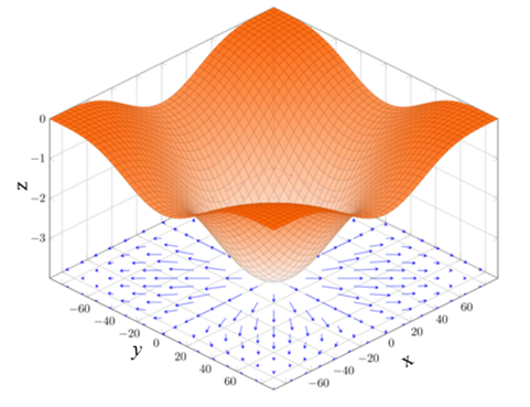
It is important to note that the gradient is a vector. It has both magnitude and direction. The direction of the gradient is the direction of the maximum directional derivative, and the magnitude of the gradient is the value of that maximum directional derivative. Geometrically, the gradient points in the direction where the function changes fastest. Moving along the gradient vector makes it easier to find the maximum value of a function. Conversely, moving in the opposite direction of the gradient vector is the direction where the function decreases fastest, so it is easier to find the minimum value. For example, the image used on Wikipedia to explain gradients is very typical and intuitive, so it is included here for reference.
[Example 1] Let \(f(x,y)=-(\cos2x+\cos2y)^{2}\). The geometric meaning of \(\mathrm{grad}f(x,y)\) can be described as a vector projection on the bottom plane. The gradient at each point is a vector. Its length represents the rate of change at that point, and its direction represents the direction in which the function increases fastest. From the gradient plot, we can clearly see that where the vectors are longer, the function increases faster. The vector direction shows the fastest direction of increase. The gradient plot is shown in Figure 1.
Now return to the concept of the loss \(\ell\). The loss \(\ell\) is also a function, such as a squared error loss function. Therefore, to find the minimum value of \(\ell\), we only need to search in the opposite direction of the gradient of \(\ell\). This is the idea of gradient descent. The formula is:
\(\mathrm{grad}=\frac{\partial\ell}{\partial\boldsymbol{\omega}_{t-1}}\)
\(\omega_t=\omega_{t\cdot1}-\eta\times\mathrm{grad}\)
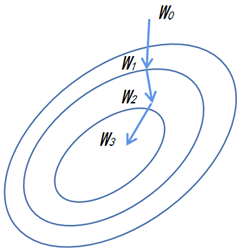
In the formula above, -grad represents the opposite direction of the gradient. The new weight \(\boldsymbol{\omega}_{t}\) equals the previous weight \(\boldsymbol{\omega}_{t-1}\) moved by \(\eta\times\mathrm{grad}\) in the opposite direction of the gradient. After the surface in Figure 1 is flattened, the gradient descent process is shown in Figure 2.
(1) Randomly initialize an initial value \(\omega_{_0}\).
(2) Repeatedly iterate the gradient descent algorithm, namely \(\boldsymbol{\omega}_{t}=\boldsymbol{\omega}_{t-1}-\eta\times\mathrm{grad}(t=1,2,3)\).
(3) At this point, the updated weight gives a smaller function value than the previous weight, namely \(\ell(\omega_0)>\ell(\omega_1)>\ell(\omega_2)\cdots\approx\ell_{\min}\).
(4) \(\eta\) is the learning rate. It describes how fast the parameters are updated. Through \(\eta\times\mathrm{grad}\), it directly affects the update speed of the parameters.
When the learning rate is too small, the update is too slow, as shown in Figure 3(a). When the learning rate is too large, gradient oscillation can easily occur, as shown in Figure 3(b). Both cases have negative effects.
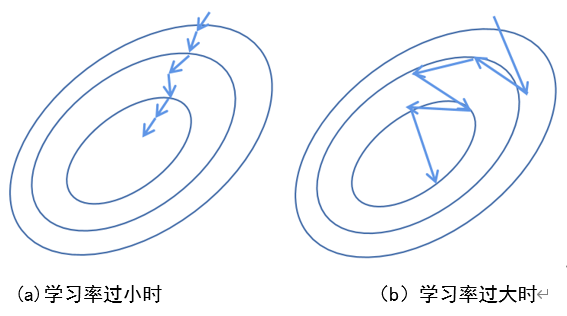
The learning rate is a key factor that directly determines whether deep learning model training succeeds. When a deep learning model performs poorly or fails to train, the reason is not always the model design. It may also be caused by the training strategy, and the learning rate is one of the main factors in that strategy. During training, we often start with a small learning rate, such as 0.0001, and then gradually increase it to observe the training result. In addition, the training dataset also directly affects model performance. In short, model performance depends on the training set, model design, and training strategy.
Finally, when training a deep learning model in a supervised setting, we usually do not use the entire dataset in one computation. The training dataset is often very large, and using all of it may exceed the available computing resources and memory. Therefore, a method called mini-batch stochastic gradient descent is commonly used. The specific method is to randomly sample \(\text{b}\) samples \(i_{1},i_{2},\cdots,i_{b}\) from the training dataset to approximate the loss. The loss is written as:
\(\frac{1}{b}\sum_{i\in I_b}\ell(x_i,y_i,\omega)\)
Here, \(\text{b}\) represents the batch size, which is an important hyperparameter in deep learning training. When \(\text{b}\) is too small, each computation is too small and cannot make full use of parallel computing resources. More importantly, a small \(\text{b}\) means that only a small subset is sampled from the training dataset. The data distribution of this subset may differ greatly from the original dataset, so it may not represent the original dataset well. When \(\text{b}\) is too large, storage or computing resources may be insufficient. According to the value of \(\text{b}\), gradient descent can be divided into Batch Gradient Descent (BGD), Stochastic Gradient Descent (SGD), and Mini-batch Gradient Descent (MBGD).
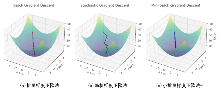
Batch Gradient Descent is a common form of gradient descent. It uses all samples to update the parameters. Because it needs to compute the gradient over the whole dataset, gradient descent may become very slow. It is also difficult when memory is limited and the dataset is large. The advantage of Batch Gradient Descent is that, under ideal conditions, it can reach the global optimum after enough iterations.
Stochastic Gradient Descent is similar in principle to Batch Gradient Descent. The difference is that SGD does not use all sample data when computing the gradient. Instead, it selects only one sample to compute the gradient. This is intended to speed up convergence and solve the problem that a large dataset cannot fit into memory at once. However, because only one sample is used to update the parameters each time, SGD can be unstable. Each update direction does not always move toward the optimum as in Batch Gradient Descent. Instead, it may oscillate around the optimum.
In fact, Batch Gradient Descent and Stochastic Gradient Descent are two extremes. The former uses all data for gradient descent, as shown in Figure 4(a). The latter uses one sample for gradient descent, as shown in Figure 4(b). The advantages and disadvantages of both methods are clear. In terms of training speed, SGD is fast because it uses only one sample in each iteration. Batch Gradient Descent can be unsatisfactory when the number of samples is large. In terms of accuracy, SGD uses only one sample to determine the gradient direction, so the result may not be optimal. In terms of convergence speed, because SGD uses one sample in each iteration, the update direction changes greatly and may not quickly converge to a local optimum. Is there a way to combine the advantages of both methods?
This is Mini-batch Gradient Descent, as shown in Figure 4(c). In each training step, a small batch of samples is randomly selected from the whole dataset for model training. The size of this mini-batch is a hyperparameter. In general, a larger batch is more accurate, but training also becomes slower.
2. Backpropagation Algorithm
Gradient descent and backpropagation are two very important concepts in neural network training, and they are closely related. Gradient descent is a commonly used optimization algorithm. Its goal is to find the minimum or maximum value of a function. In neural networks, gradient descent adjusts the weights of each neuron to minimize the network’s loss function. The loss function measures the error between the network output and the true value. The core idea of gradient descent is to compute the partial derivative of the loss function with respect to the weights, and then adjust the weights in the opposite direction of this partial derivative.
Backpropagation is an efficient method for computing gradients. It can quickly compute the partial derivative for each neuron in the network. Backpropagation first computes the network output through forward propagation. Then it propagates the error backward from the output layer to the input layer. Finally, it computes the partial derivative of each neuron based on the error. The core idea of backpropagation is to pass the error backward through the chain rule and compute each neuron’s contribution to the error.
In summary, gradient descent and backpropagation are two important concepts in neural network training. Gradient descent is used to optimize the network weights, while backpropagation is used to compute the partial derivatives of each neuron. They are closely related and play important roles in neural network training.
[Example 2] The complete process of updating the parameters of a neural network layer.
(1) Initialize the network and build a neural network with only one layer, as shown in Figure 5.
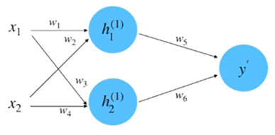
Assume that the input and output of the neural network in Figure 5 are initialized as \(x_{1}=0.5,x_{2}=1.0,y=0.8\). The parameters are initialized as \(w_{1}=1.0,w_{2}=0.5,w_{3}=0.5,w_{4}=0.7,w_{5}=1.0,w_{6}=2.0\).
(2) Forward computation, as shown in Figure 6.
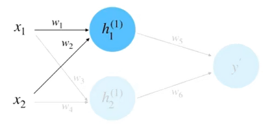
Compute \(h_{1}\) from the inputs and weights:
\(\begin{aligned}h_{1}^{(1)}&=w_1\cdot x_1+w_2\cdot x_2\\&=1.0\cdot0.5+0.5\cdot1.0\\&=1.0\end{aligned}\)
Similarly, \(h_{2}\) is 0.95. Multiply and sum \(h_{1}\) and \(h_{2}\) to obtain the forward propagation result, as shown in Figure 7.
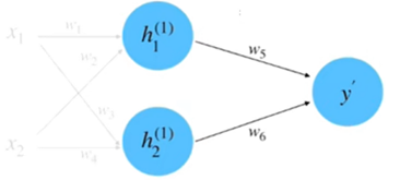
\(\begin{aligned}y^{\prime}&=w_{5}\cdot h_{1}^{(1)}+w_{6}\cdot h_{2}^{(1)}\\&=1.0\cdot1.0+2.0\cdot0.95\\&=2.9\end{aligned}\)
(3) Compute the loss. Use the true value \(y=0.8\) and the squared error loss function to compute the loss, as shown in Figure 8.
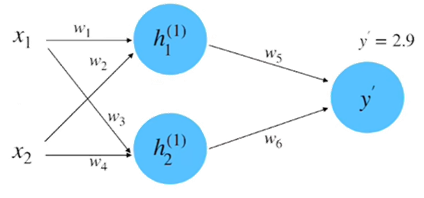
\(\begin{aligned}\delta&=\frac{1}{2}(y-y^{\prime})^{2}\\&=0.5(0.8-2.9)^{2}\\&=2.205\end{aligned}\)
(4) Compute the gradient. This process is essentially the computation of partial derivatives. Take the partial derivative with respect to parameter \(w_{5}\) as an example, as shown in Figure 9.
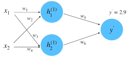
According to the chain rule:
\(\frac{\partial\delta}{\partial w_5}=\frac{\partial\delta}{\partial y^{\prime}}\cdot\frac{\partial y^{\prime}}{\partial w_5}\)
where:
\(\begin{aligned}\frac{\partial\delta}{\partial y^{\prime}}&=2\cdot\frac{1}{2}\cdot(y-y^{\prime})(-1)\\&=y^{\prime}-y\\&=2.9-0.8\\&=\begin{array}{c}{2.1}\end{array}\end{aligned}\)
\(y^{\prime}=w_5\cdot h_1^{(1)}+w_6\cdot h_2^{(1)}\)
\(\begin{aligned}\frac{\partial y^{\prime}}{\partial w_{5}}&=h_{1}^{(1)}+0\\&=1.0\end{aligned}\)
Therefore:
\(\frac{\partial\delta}{\partial w_5}=\frac{\partial\delta}{\partial y^{\prime}}\cdot\frac{\partial y^{\prime}}{\partial w_5}=2.1\times1.0=2.1\)
(5) Use backpropagation to compute the gradient. In Step 4, parameter \(w_{5}\) was used as an example to compute a partial derivative. If we use parameter \(w_{1}\) as an example, its partial derivative requires the chain rule. The process is shown in Figure 10.
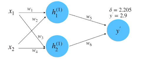
\(\frac{\partial\delta}{\partial w_{1}}=\frac{\partial\delta}{\partial y^{\prime}}\cdot\frac{\partial y^{\prime}}{\partial h_{1}^{(1)}}\cdot\frac{\partial h_{1}^{(1)}}{\partial w_{1}}\)
\(y^{\prime}=w_5\cdot h_1^{(1)}+w_6\cdot h_2^{(1)}\)
\(\begin{aligned}\frac{\partial y^{\prime}}{\partial h_1^{(1)}}&=w_5+0\\&=1.0\end{aligned}\)
\(h_1^{(1)}=w_1\cdot x_1+w_2\cdot x_2\)
\(\begin{aligned}\frac{\partial h_1^{(1)}}{\partial w_1}&=x_1+0\\&=0.5\end{aligned}\)
\(\frac{\partial\delta}{\partial w_1}=\frac{\partial\delta}{\partial y^{\prime}}\cdot\frac{\partial y^{\prime}}{\partial h_1^{(1)}}\cdot\frac{\partial h_1^{(1)}}{\partial w_1}=2.1\times1.0\times0.5=1.05\)
(6) Use gradient descent to update the network parameters.
Assume that the initial value of the hyperparameter “learning rate” is 0.1. According to the gradient descent update formula, the update for parameter \(w_{1}\) is:
\(w_1^{(\mathrm{update})}=w_1-\eta\cdot\frac{\partial\delta}{\partial w_1}=1.0-0.1\times1.05=0.895\)
Similarly, the other updated parameters can be computed as:
\(w_1=0.895,w_2=0.895,w_3=0.29,w_4=0.28,w_5=0.79,w_6=1.8005\)
At this point, we have completed the full process of one parameter iteration. We can compute the loss to see whether it has decreased:
\(\begin{aligned}\delta=&\frac{1}{2}(y-y^{\prime})^{2}\\&=0.5(0.8-1.3478)^{2}\\&=0.15\end{aligned}\)
Compared with the previous forward propagation loss of 2.205, this result is significantly smaller.
SGD Optimizer
Stochastic Gradient Descent (SGD) is an optimization algorithm widely used to train machine learning models. Its core idea is to compute the gradient of the loss function with respect to the model parameters and update the parameters in the opposite direction of the gradient, so that the loss function is minimized. SGD uses only one sample or one small batch of samples in each update, so it is computationally efficient. However, it may converge slowly and suffer from oscillation. To address these problems, Momentum has become one of the key techniques in SGD. Momentum introduces information from historical gradients and accumulates previous update directions. This accelerates convergence, reduces oscillation, and makes the optimization process more stable and efficient.
During gradient descent, an exponential moving average is used to combine historical gradients. This brings clear benefits for convergence speed and stability. The historical gradient term is called the Momentum term. The optimization steps of SGD with momentum are:
\(m_t=\beta m_{t-1}+(1-\beta)g_t\)
\(\omega_{t}=\omega_{t-1}-\eta m_{t}\)
Here, \(m_{_{t-1}}\) is the gradient from the previous time step, \(m_{_{t}}\) is the gradient after historical gradients are combined with EMA, and \(\mathbf{g}_{t}\) is the current gradient. \(\mathrm{β}\) is a hyperparameter, and \(\beta m_{_{t-1}}\) is called the Momentum term. From the principle of EMA, although the formula only uses the gradient from the previous time step, it is actually an exponential average of all historical gradients before the current time step.
After adding the Momentum term, model weight updates are smoother and more stable than directly using the raw gradient. Momentum can also help the optimization quickly pass through flat regions on the error surface, such as saddle points. The idea can be imagined as skiing. The current movement trend is always affected by previous kinetic energy, so the skiing path is smooth and graceful. It cannot suddenly make a sharp 90° right-angle turn. When the skier reaches the bottom of a valley, the terrain is flat, but because of previous kinetic energy, the skier may continue moving forward and may even use the momentum to move out of the valley.
In summary, adding Momentum has the following benefits:
(1) In the early stage of descent, the Momentum direction is consistent with the current gradient direction, which can accelerate convergence well.
(2) In the later stage of descent, the gradient may oscillate near a local minimum, and Momentum may help escape the local minimum.
(3) When the gradient changes direction, Momentum can offset gradients in opposite directions, suppress oscillation, and speed up convergence.
Gradient descent with Momentum also has another simple implementation:
\(g_{i}=\beta g_{i-1}+g(\theta_{i-1})\)
\(\theta_i=\theta_{i-1}-\alpha\boldsymbol{g}_i\)
AdaGrad Optimizer
Momentum is one way to optimize mini-batch gradient descent. Another method is called the AdaGrad algorithm. It mainly further optimizes the learning rate. The parameter update formula is:
\(r_{_k}\leftarrow r_{_{k-1}}+g\odot g\)
\(\theta_{_k}\leftarrow\theta_{_{k-1}}-\frac{\eta}{\sqrt{r_{_k}+\sigma}}\odot g\)
From the formula above, compared with ordinary gradient descent, $\eta$ becomes \(\frac{\eta}{\sqrt{r_i+\sigma}}\), where \(\sigma\) is a very small real number used to prevent division by zero. \(r_{k}\) is the accumulated value of the squared gradients from previous time steps. Here we consider two questions:
- Why should the gradient be squared?
- Why should the squared gradients be accumulated?
The role of the squared gradient is to smooth the current gradient. If \(\mathrm{g}\) is small, then \(g\odot g\) becomes even smaller, so \(r_{k}\) is small and \(\frac{1}{\sqrt{r_{i}+\sigma}}\) is relatively large. In this case, the learning rate \(\eta\) is effectively amplified. Conversely, if \(\mathrm{g}\) is large, the learning rate \(\eta\) is reduced.
Accumulating historical gradients is intended to make the learning rate gradually decrease as training proceeds. Because of the accumulation, \(r_{k}\) becomes larger and larger, and \(\frac{\eta}{\sqrt{r_k+\sigma}}\) becomes smaller as training continues. This is a suitable learning rate adjustment strategy. It is like playing golf. We can think of the learning rate as the force used to swing the club. At the beginning, we use more force because we want the ball to quickly approach the hole. Near the end, we use less force and slowly hit the ball into the hole.
Of course, AdaGrad also has disadvantages. First, the formula shows that it still depends on a manually set global learning rate. Second, if \(\eta\) is set too large, \(\sqrt{r_{k}+\sigma}\) becomes too sensitive, and the adjustment to the gradient becomes too strong. Finally, in the middle and late stages of training, the accumulated squared gradients in the denominator become larger and larger, causing \(\mathrm{gradient}\to0\). This may stop training too early.
RMSprop Optimizer
RMSprop is a development of AdaGrad. It works well for recurrent neural networks. In essence, it introduces the idea of EMA into \(r_{k}\). The formula is:
\(r_{_k}\leftarrow\beta r_{_{k-1}}+(1-\beta)g\odot g\)
\(\theta_{_k}\leftarrow\theta_{_{k-1}}-\frac{\eta}{\sqrt{r_{_k}+\sigma}}\odot g\)
The goal is to give recent gradients greater weight when accumulating squared historical gradients, instead of accumulating them endlessly and eventually making the gradient become 0. Although RMSprop can automatically adjust the learning rate better, it still depends on the initial setting of the global learning rate.
Adam Optimizer
Finally, Adam can be regarded as the most commonly used optimization algorithm in deep learning. It combines the advantages of other optimization algorithms. It can be seen as an RMSprop optimizer with Momentum, and it further improves on this basis to avoid the cold-start problem. Its computation process is as follows:
Input: learning rate \(\varepsilon\), initial parameters \(\theta\), small constant \(\mathrm{σ}\), accumulated gradient \(_{\nu}\), accumulated squared gradient \(\mathrm{r}\), decay coefficient \(\rho\), and Momentum parameter \(\alpha\).
Sample \(\mathrm{m}\) examples $\lbrace{x^1, x^2, \ldots, x^m} \rbrace$ from the training set. Use data \(x^{(i)}\) and the corresponding target \(y^{(i)}\) to compute the gradient:
\(g\leftarrow\frac{1}{m}\nabla_{\theta_{k-1}}L(f(x^{(i)},\theta_{_{k-1}}),y^{(i)})\)
Compute the accumulated gradient: \(v_{t}=\alpha v{_{t-1}}+(1-\alpha)g\), that is, add the Momentum term.
Compute the accumulated squared gradient: \(r_{t}=\rho r_{t-1}+(1-\rho)g\odot g\), that is, adjust the learning rate through the RMSprop algorithm.
Correction: \(\hat{\nu}{t}=\frac{\nu{t}}{1-\alpha}\), \(\hat{r}{t}=\frac{r{t}}{1-\rho}\).
Update the parameters: \(\theta_{k}\leftarrow\theta{{k-1}}-\varepsilon\frac{\hat{v}{t}}{\sqrt{\hat{r}{_t}+\sigma}}\)
Here is an explanation of the cold-start problem. Assume that the decay coefficient is 0.999 and the Momentum parameter is 0.9.
Then, at the beginning of training:
\(v=0.9\times0+0.1\times g=0.1g\)
\(r=0.999\times0+0.001\times g^2=0.001g^2\)
\(\text{r}\) and \(\nu\) are both very small at the start of training. This means that the initial training gradient is small and parameter updates are slow. After correction:
\(V=\frac{v}{1-0.9}=\frac{0.1\boldsymbol{g}}{0.1}=\boldsymbol{g}\)
\(R=\frac{r}{1-0.999}=\frac{0.001\boldsymbol{g}^2}{0.001}=\boldsymbol{g}^2\)
This method can reduce the cold-start problem to some extent.