
1. Overfitting and Underfitting During Optimization
Overfitting and underfitting are two common problems that can appear when training deep learning models.
Underfitting happens when the model is less expressive than the true pattern in the data. A suitable solution for a nonlinear problem is shown in Figure 1(a). If we use a linear model to train on this nonlinear problem, it is naturally difficult to obtain a good solution, as shown in Figure 1(b).

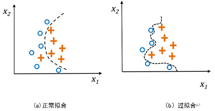
In contrast, overfitting happens when the model is more expressive than the true pattern in the data. To improve accuracy on the training set, the model learns too many non-general features. This reduces its generalization ability. The model can fit the training set well, but it performs poorly on the test set. A normally fitted model is shown in Figure 2(a), and an overfitted model is shown in Figure 2(b).
There are two main factors that affect overfitting and underfitting: the data, especially the amount of data, and the model capacity, or model complexity. Their relationship is shown in Table 1.
| Simple data | Complex data | |
| Low model capacity | Normal fit | Underfitting |
| High model capacity | Overfitting | Normal fit |
From the perspective of data volume, overfitting is more likely when there is too little training data. Underfitting is more likely when the data is too large or too difficult for the model. We can explain this with a simple example. Suppose a university student is preparing for a final exam. If the practice question bank, which acts like the training set, is too simple, the student may prepare by memorizing the answers. The student may even remember all answers from previous exams, but this does not mean that the student truly understands the questions. This situation, where every sample in the training set is memorized, is called overfitting. In contrast, if the practice question bank is too large and too difficult, it may exceed what the student can remember. The student may also fail to understand the relationships between questions or analyze the features of the data. In this case, the training set is too difficult, and the model cannot handle the task. This is called underfitting.
From the perspective of model complexity, why would a university student think of memorizing answers? If a kindergarten child were asked to solve the same problems, would the child think of this method? A university student can be compared to a complex model, while a kindergarten child can be compared to a simple model. From this, we can easily see that a complex model is more likely to overfit, because it is more capable of memorizing each sample in the training set instead of learning general features.
Training error and generalization error are two important indicators for measuring how well a model fits. First, let us define them:
(1) Training Error: the error computed on the training dataset.
(2) Generalization Error: the expected model error when the model is applied to infinitely many data samples drawn from the same distribution as the original samples.
The problem is that we can never compute the generalization error exactly. Infinitely many data samples are only an idealized object. In practice, we estimate the generalization error by applying the model to an independent test set. This test set is composed of randomly selected samples that did not appear in the training set.
A clear sign of overfitting is that the model has a small training error but a large generalization error. Underfitting is reflected by both a large training error and a large generalization error. The goal of training a model is to make it work in the real world. In other words, we want a small generalization error. Therefore, both overfitting and underfitting should be avoided when training deep learning models.
Overfitting can also be explained from the perspective of the “curse of dimensionality.” In the deep learning models introduced earlier, each neural network layer may contain a different number of perceptrons. This is equivalent to increasing or reducing the dimensionality of the original data and extracting features in spaces with different dimensions. What does a space with different dimensions mean? Consider a simple example. Suppose we use a linear classifier to perfectly classify cats and dogs. We may start with one feature, such as “round eyes.” The classification result is shown in Figure 3.

Because both cats and dogs have round eyes, we cannot obtain a perfect classification result at this point. Therefore, we may decide to add another feature, such as “pointed ears.” The classification result is shown in Figure 4.
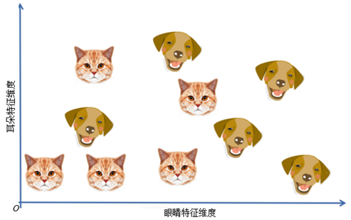
Now the data distributions for cats and dogs gradually become more separated. Finally, we add a third feature, such as “long nose,” and obtain a three-dimensional feature space, as shown in Figure 5.
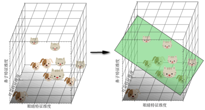
At this point, the model can already fit a classification decision surface that separates cats and dogs well. This naturally leads to a question: if we continue to add more features and map the original data into a higher-dimensional space, will classification become easier?
This is not true. Notice that when the dimensionality of the problem increases, the density of training samples decreases exponentially. Suppose 10 training examples cover the complete one-dimensional feature space, whose width is 5 unit intervals. In the one-dimensional case, the sample density is therefore (10/5 = 2) samples per interval.
In the two-dimensional case, we still have 10 training examples. Now they cover a two-dimensional feature space with an area of 5 × 5 = 25 unit squares. Therefore, the sample density is (10/25 = 0.4) samples per interval.
Finally, in the three-dimensional case, 10 samples cover a feature-space volume of 5 × 5 × 5 = 125 unit cubes. Therefore, the sample density is (10/125 = 0.08) samples per interval.
If we keep adding features, the number of dimensions in the feature space continues to grow, and the space becomes increasingly sparse. Because of this sparsity, it becomes very easy to find a separable hyperplane. In this case, the classification decision surface learned by the model can separate all individual training samples very easily and perfectly. Some readers may ask: is it not good to perfectly separate the training data?
In fact, it is not. Training data comes from the real world, and no training set can contain every possible real-world case. For example, when collecting a dataset of cats and dogs, it is impossible to photograph every cat and dog in the world. Perfectly separating this training dataset may actually fix the model’s thinking too rigidly, making its generalization ability poor in the real world. In daily life, this is like getting stuck in a narrow definition. For example, suppose we spend a great deal of effort defining Chinese cattle using one hundred features. This strict definition can easily distinguish cattle from other species. But one day, a British dairy cow crosses the ocean and arrives in China. Because this foreign cow satisfies only 90 of the features in the Chinese definition of cattle, it is not classified as a cow. This is clearly unreasonable. The reason is that the feature-space dimension is too high. This phenomenon is called the “curse of dimensionality.” When the dimensionality of a problem becomes large, classifier performance decreases. The curse of dimensionality is illustrated in Figure 6.

The next question is: how large is “large,” and how can we avoid the curse of dimensionality? Unfortunately, there is no fixed rule for deciding how many features should be used in classification. In fact, it depends on the amount of available training data, the complexity of the decision boundary, and the type of classifier used. If a theoretically infinite amount of training data were available, the curse of dimensionality would disappear.
In practice, we usually accept the following fact: if we increase the feature dimension extracted from the data, or if the model requires higher-dimensional input, we also need to increase the amount of training data. For example, when features are manually extracted, combining multiple features often means that more data is needed to train the final model. Similarly, in deep neural networks, the input dimension is often high, so a large amount of training data is usually required. Otherwise, the model will not have enough data to learn from.
Looking back at the previous example, the expansion of the high-dimensional feature space makes the original samples sparse. Samples that were originally close to each other may become very far apart. This curse of dimensionality increases the risk of overfitting. As data dimensionality increases, the model is more likely to learn noise in the training data rather than its true structure.
Preventing overfitting is essential for building deep learning models that can generalize to new data. An overfitted model may perform very well on training data, but it usually performs poorly on unseen data. This limits its usefulness and reliability. Common ways to avoid overfitting include regularization, Dropout, and data augmentation.
L1 regularization is a technique used in machine learning and statistics to prevent model overfitting. It works by adding a penalty term to the loss function that is proportional to the absolute values of the model parameters. Suppose we have a simple neural network composed of an input layer, two hidden layers, and an output layer. The weight matrix between each pair of layers is denoted by \(\mathrm{W}\).
Let the output of the neural network be \(h(W,x^{(i)})\), and let the true value be \(y^{(i)}\). The MSE loss function is defined as:
\(J_{MSE}(W)=\frac{1}{m}\sum_{i=1}^{m}\left(h(W,x^{(i)})-y^{(i)}\right)^{2}\)
Here, \(\mathrm{m}\) is the number of training samples, and \(\mathbf{W}\) represents all weights in the neural network.
When L1 regularization is added, the loss function becomes:
\(J_{L1}(\boldsymbol{W})=\frac{1}{m}\sum_{i=1}^{m}\left(h(\boldsymbol{W},\boldsymbol{x}^{(i)})-\boldsymbol{y}^{(i)}\right)^{2}+\lambda\sum_{l}\sum_{i}\sum_{j}\left|\boldsymbol{W}_{ij}^{(l)}\right|\)
The extra term outside the original loss function is the L1 regularization term. During loss minimization, the regularization term and the original loss are added together, so both gradually decrease during training. Because the regularization term is the sum of the absolute values of all parameters, reducing this term means limiting all parameters in the model so that they do not become too large. This helps prevent unstable gradients during training. Note that \(\lambda\) is the regularization strength parameter. \(W_{ij}^{(l)}\) is an element of the weight matrix in the \(\mathrm{l}\)-th layer, connecting the \(\mathrm{i}\)-th neuron to the \(\mathrm{j}\)-th neuron. The outer summations cover all layers, all neurons, and their connections in the network.
L1 regularization has the following effects:
(1) Weight sparsity: L1 regularization makes many weights in the network approach 0, which introduces sparsity into the weights.
(2) Model simplification: because some weights become 0, some connections in the network are effectively “turned off.” This helps reduce overfitting and simplifies the model.
As mentioned earlier, choosing an appropriate regularization strength, namely the value of \(\lambda\), is critical. If the value is too small, the regularization effect may be weak. If it is too large, too many weights may become 0, which can oversimplify the model. Cross-validation is usually a good way to determine the best value of \(\lambda\).
In comparison, L2 regularization adds a squared absolute-value term of \(\boldsymbol{\omega}\) to the loss function. This encourages \(\boldsymbol{\omega}\) to stay as small as possible. L2 regularization usually does not regularize the parameter b. It only includes the regularization of \(\boldsymbol{\omega}\), because b has few parameters, is unlikely to increase model complexity, and is unlikely to increase the variance of the model output. Regularizing b may instead cause underfitting. After adding L2 regularization to the loss function, the new loss function \(L^{\prime}\) is written as:
\(L^{\prime}=L+\frac{1}{2}\lambda\|\boldsymbol{\omega}_{t-1}\|^2\)
Taking the derivative of the loss function \(L^{\prime}\) gives the derivative \(g^{\prime}\):
\(g^{\prime}=g+\lambda\boldsymbol{\omega}_{t-1}\)
Using gradient descent to update the parameter \(\boldsymbol{\omega}_{t}\):
\(\omega_t=\omega_t-\eta g-\eta\lambda\omega_{t-1}=(1-\eta\lambda)\boldsymbol{\omega}_t-\eta\boldsymbol{g}\)
Usually, \(\eta\lambda<1\). Therefore, when it is multiplied by the parameter \(\boldsymbol{\omega}_{t}\), it has the effect of decaying the weight. For this reason, L2 regularization is also called weight decay.
Regularization can be viewed as a set of methods that prevent overfitting by constraining model complexity. Model complexity is determined by both the number of model parameters and the range of values those parameters can take. Therefore, regularization methods can be divided into two directions. One direction constrains the value range of model parameters, as in the regularization methods above. The other direction constrains the number of model parameters, such as Dropout, shown in Figure 7. A network without Dropout is shown in Figure 7(a), and a network processed by Dropout is shown in Figure 7(b). During training, Dropout randomly sets the outputs of nodes in each neural network layer to zero with a certain probability. In implementation, all weights connected to the dropped neurons are set to zero. These dropped neurons are not activated or updated during the forward propagation and backpropagation of the current training sample.
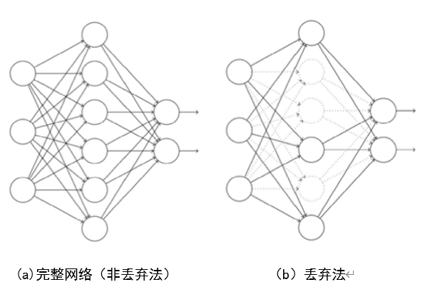
From Figure 7, we can see that after Dropout is applied, the number of model parameters is significantly reduced. This reduces model complexity.
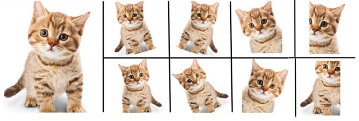
All the methods above prevent overfitting from the perspective of model complexity. Next, we explain how to prevent overfitting from the perspective of training-set size. This type of method is called data augmentation. The idea is simple: increasing the number of samples in the training dataset can help prevent overfitting. Take computer vision tasks as an example. We can take each sample from an image dataset and apply different random crops, horizontal flips, color and lighting changes, contrast adjustments, and other operations. In this way, many copied variants can be generated from one original image. These images are then used together as the model’s training set, increasing the dataset capacity. An example is shown in Figure 8.
Of course, this simple approach is already relatively old. Today, we can also use generative deep learning models, such as generative adversarial networks (GANs), to generate new samples as training samples. Experiments have shown that this is feasible.
At this point, we have introduced three ways to prevent overfitting during deep learning training: regularization, Dropout, and data augmentation. Methods for preventing underfitting are simpler: increase model complexity. For example, we can directly increase the number of hidden layers in the deep learning model to make it deeper, or increase the number of nodes in each neural network layer to make it wider.
2. Gradient Instability During Optimization
A deep learning model is a neural network formed by stacking layers. During forward propagation, each neural network layer essentially performs multiplication and summation. Therefore, the computation in a deep model with many stacked layers is essentially a repeated multiplication process. During backpropagation, because the chain rule is used, this repeated multiplication property still exists. Repeated multiplication can cause numerical instability. In deep learning training, this numerical instability directly leads to two problems in gradient propagation:
(1) Vanishing gradients: in deep neural networks, gradient diffusion means that gradients gradually become smaller during backpropagation until they are close to zero in the shallow layers of the network. As a result, the weights in these layers are barely updated, making it difficult for the model to learn complex features from the input data.
(2) Exploding gradients: in contrast, exploding gradients mean that gradients become abnormally large during backpropagation. This causes excessive weight updates, making model parameters extremely unstable and possibly causing numerical overflow. The model may fail to converge, and the violent weight updates during training can sharply reduce model performance.
One way to prevent gradient instability is to normalize the data. This means normalizing each training mini-batch, which is called Batch Normalization (BN). BN appears frequently in later network models and has become an essential component of neural networks. Next, we explain the principle of BN from the perspective of training.
During network training, the parameters keep changing, so the input distribution of each later layer also changes. The learning process must make each layer adapt to its input distribution. As a result, we often have to reduce the learning rate and initialize parameters carefully. This change in distribution is called internal covariate shift (ICS). To solve this problem, researchers proposed a solution: subtract the mean from the input data during network training. The purpose of this operation is to speed up network training.
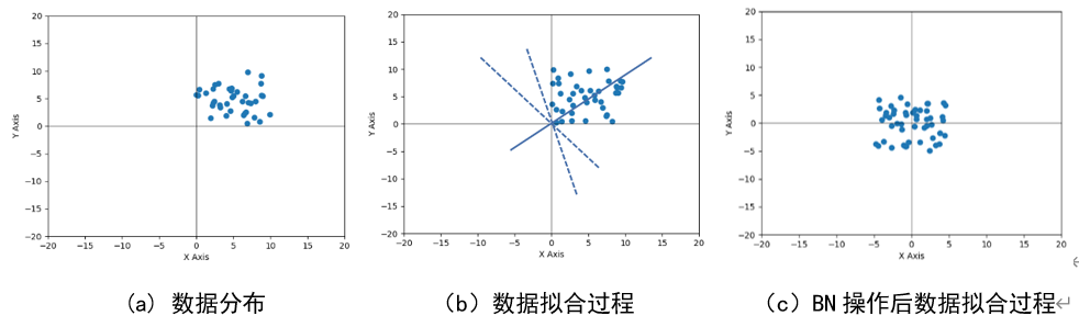
Why can mean subtraction speed up training? Here is a simple explanation. Image data is highly correlated, and similar images are close to each other when represented as data distributions in a high-dimensional space. Suppose the distribution is as shown in Figure 9(a), where each point represents an image and the case is simplified to two dimensions. During initialization, parameters usually have zero mean. Therefore, the initial fit \(y=\omega x+b\) is basically near the origin, as shown by the line in Figure 9(b). The network must go through many learning steps before it gradually reaches the fit shown by the solid line, so convergence is slow. If we subtract the mean from the input data first, learning can clearly be accelerated, as shown in Figure 9(c).
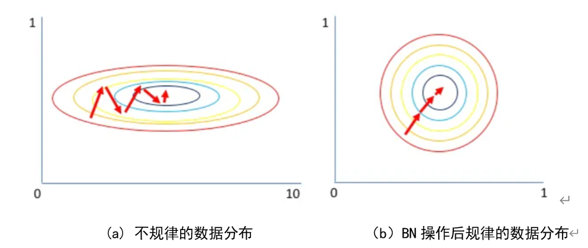
A visual explanation is that BN normalizes the data distribution of the input to each neural network layer. It changes an irregular data distribution, as shown in Figure 10(a), into a regular data distribution, as shown in Figure 10(b). The arrows indicate the process by which the model searches for the optimal solution. Clearly, the situation in Figure 10(b) is more convenient and easier.
Finally, the formula for BN is as follows:
Input information: the values of \(\mathrm{x}\) in the mini-batch \(B={x_{1..m}}\); learnable parameters: \(\mathrm{r}\) and \(\beta\);
Output information: \({y_{i}=BN_{{\gamma,\beta}}(x{_i})}\).
The algorithm is as follows:
\(\mu_s\leftarrow\frac{1}{m}\sum_{i=1}^mx_i\) (1)
\(\sigma_{_B}^{^2}\leftarrow\frac{1}{m}\sum_{i=1}^{^m}(x_{_i}-\mu_{_B})^2\) (2)
\(\hat{X}_1\leftarrow\frac{X_\mathrm{i}-\mu_\mathrm{\beta}}{\sqrt{\sigma_\mathrm{\beta}^2+\epsilon}}\) (3)
\(y_i\leftarrow\hat{\gamma}x_i+\beta\equiv BN_{\beta,\gamma}(x_i)\) (4)
Equation (1) computes the mean \(\mu\) of each batch along the channel dimension. Equation (2) computes the variance \(\sigma^{2}\) of each batch along the channel dimension. Equation (3) normalizes \(\mathrm{x}\) as \(x^{\prime}=(x-\mu)/\sqrt{\sigma^{2}+\varepsilon}\). Finally, Equation (4) adds the scaling and shifting variables \(\mathrm{r}\) and \(\beta\). The reason for adding scaling and shifting variables to the normalized value, \(y=\gamma x^{\prime}+\beta\), is that the data may not always need to follow a standard normal distribution. It may need shifting or stretching. This ensures that after each normalization step, the data still preserves the features learned by the model while also completing normalization and accelerating training. These two parameters are learnable and can be updated as the network is trained.
In addition to gradient instability caused by repeated multiplication, improper network parameter initialization and unsuitable activation functions can also lead to gradient instability. For example, in vanishing gradients, activation functions such as Sigmoid or Tanh have derivatives that approach zero when the input value is very high or very low. This causes gradients to become smaller layer by layer. In exploding gradients, weights initialized too large or activation functions without an upper saturation limit, such as ReLU, may cause gradients to grow exponentially as the number of layers increases. Therefore, some work focuses on improving activation functions. Examples include ReLU variants such as Leaky ReLU, Swish, and ReLU6. These variants provide a nonzero slope in the negative region, reducing gradient disappearance for negative inputs. They also limit the maximum value in the positive region to prevent exploding gradients caused by repeated multiplication. These measures help keep gradients flowing healthily through the whole network, especially in deep networks. Finally, reasonable network parameter initialization can also help gradients propagate well. For example, He initialization is especially suitable for networks using ReLU activation functions, while Xavier initialization is suitable for networks using Sigmoid and Tanh activation functions. We will not expand on these details here.