 Deep Learning Math
Advanced Mathematics
Advanced mathematics plays a crucial role in deep learning. The foundations of calculus, such as integration and differentiation, help us understand the model-training process. Through derivatives and the monotonicity of functions, we can judge the direction of optimization, and we can use the chain rule to compute gradients of complex functions. Gradient descent is at the heart of deep-learning optimization: it minimizes the loss function by computing gradients. Extrema and saddle points, the Hessian matrix, and the concavity and convexity of functions help us understand a model’s behavior and stability during optimization. In addition, Taylor expansions and Fourier series are used for function approximation and signal processing, which are especially important when building and optimizing complex neural-network models. With these mathematical tools, deep-learning models can be trained and optimized more effectively, improving both performance and accuracy.
 Agenda
- Calculus
- Integration
- Differentiation and Derivatives
- Monotonicity of Functions
- Extrema and Saddle Points of Functions
- Hessian Matrix
- Concavity and Convexity of Functions
- Chain Rule
- Gradient
- Taylor Series / Taylor Expansion
- Fourier Series
 Calculus
Calculus is a branch of mathematics that primarily studies quantities that change and the relationships between them. It consists of two main parts: differential calculus and integral calculus.
- Differential calculus focuses on rates of change and slopes of functions. Its main tool is the derivative, which describes the speed of instantaneous change.
- Integral calculus focuses on accumulated quantities. Its main tool is the integral, which is used to compute areas, volumes, and other accumulated quantities.
 Integration
- Geometric interpretation of integration: the area under the curve of a function.
- Physical interpretation of integration: the physical meaning of an integral depends on the quantity being integrated. For example, integrating force over time gives the impulse over a period of time; integrating force over space gives the work done by that force over a displacement.
- Algebraic interpretation of integration: a more refined form of multiplication.
How should we understand integration as a more refined form of multiplication? Let’s return to the physical system of distance, speed, and time as an example:
Suppose the current velocity is $v=5 \mathrm{~m} / \mathrm{s}$ and the time is $t=10 \mathrm{~s}$. How do we find the distance traveled, $s$?
- This is easy: ordinary multiplication is enough, $(s=v t)$. But there is one prerequisite: the velocity must be constant.
What if the velocity is changing? That is where integration comes in.
- Suppose the velocity is now $v=2 t$. What is the distance traveled by the 10th second?
The idea of integration is to divide the time interval into segments as small as possible, use the instantaneous velocity at the start of each segment as the average velocity over that segment, and finally add up the distances traveled in all these small segments to obtain the total distance traveled in 10 seconds.
The specific solution is as follows:
- At $1 \mathrm{~s}$, the car’s velocity is $v_1=2 t=2 \cdot 1=2(\mathrm{~m} / \mathrm{s}) ;$
- At $2 \mathrm{~s}$, the car’s velocity is $v_2=2 t=2 \cdot 2=4(\mathrm{~m} / \mathrm{s})$;
- At $3 \mathrm{~s}$, the car’s velocity is $v_3=2 t=2 \cdot 3=6(\mathrm{~m} / \mathrm{s})$;
- Continuing in this way,
- At $10 \mathrm{~s}$, the car’s velocity is $v_{10}=2 t=2 \cdot 10=20(\mathrm{~m} / \mathrm{s})$.
- Then use multiplication to compute the distance for each small time segment $(t=1 \mathrm{~s})$, namely:
$$
\begin{aligned}
s & =\sum_{i=1}^{10} s_i \\
& =s_1+s_2+s_3+\cdots+s_{10} \\
& =2+4+6+\cdots+20 \\
& =\frac{10(2+20)}{2} \\
& =110 \\
\end{aligned}$$
In the formula above, the 10 seconds are divided into 10 one-second intervals, and the final distance obtained is 110 m. The visualization is shown below.
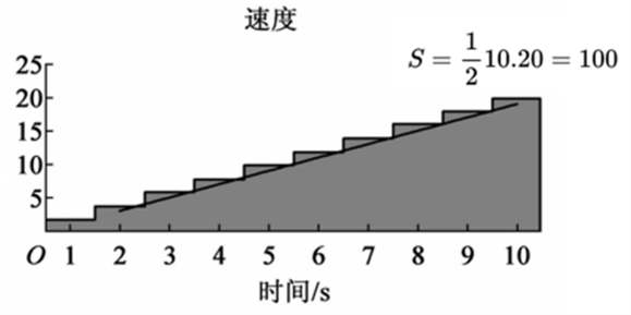
You can imagine that when the time interval is small enough, the graph of this velocity function is approximately a triangle. The distance is then the area of that triangle, which is 100 m. The rough estimate of 110 m obtained above is already very close to the correct answer.
So the essence of integration is more refined multiplication: after summing the pieces, we obtain the output result.
In deep learning, integration is used far less often than differentiation, so this section gives only a brief conceptual introduction. The following discussion focuses on differentiation.
 Differentials and Derivatives
Differentials and derivatives are both related to rates of change of functions. They are related concepts, but they are not exactly the same. Let’s first take a closer look at their definitions and differences.
-
A derivative describes the slope of the tangent line to a function at a point. If we have a function $y=f(x)$, then its derivative at the point $x$ is usually written as $f^{\prime}(x)$ or $\frac{\mathrm{d} y}{\mathrm{~d} x}$. The derivative is defined as the limit of the average rate of change at that point, as follows:
$$
f^{\prime}(x)=\lim _{\Delta x \rightarrow 0} \frac{f(x+\Delta x)-f(x)}{\Delta x}$$ -
A differential describes the relationship between a tiny change in the function value and a tiny change in the independent variable. For a function $y=f(x)$, its differentials are denoted by $\mathrm{d} y$ and $\mathrm{d} x$, where $\mathrm{d} y$ is the tiny change in the function value and $\mathrm{d} x$ is the tiny change in the independent variable. The definition of the differential is based on the derivative and can be written as:
$$
\mathrm{d} y=f^{\prime}(x) \cdot \mathrm{d} x$$
Thus, derivatives and differentials are both related to rates of change, but their emphases are slightly different. A derivative focuses on the slope of the tangent line at a point, while a differential focuses on the relationship between a tiny change in the function value and a tiny change in the independent variable.
In short, a derivative is a concept of ratio or slope, whereas a differential describes how the dependent variable changes when the independent variable changes by a very small amount.
Derivatives as Refined Division
- Geometric interpretation of the derivative: the slope of the tangent line to the function curve at that point.
- Physical interpretation of the derivative: the physical meaning of a derivative depends on the quantity involved, but it always describes how fast that quantity changes—that is, its rate of change.
- Algebraic interpretation of the derivative: a more refined form of division.
The first two interpretations are probably familiar. But how should we understand the claim that the derivative is, algebraically, a more refined form of division?
Consider a physical example:
Distance $s=25 \mathrm{~m}$, time $t=5 \mathrm{~s}$. What is the average velocity $v$?
This is easy to answer: ordinary division handles it directly ( $v=s / t)$.
But if the velocity is not uniform, and we want the instantaneous velocity at the 5th second, what should we do?
$$
v=\left.\frac{\mathrm{d} s}{\mathrm{~d} t}\right|_{t=5}=\lim _{\Delta t \rightarrow 0} \frac{s(5+\Delta t)-s(5)}{\Delta t}$$
$\Delta t$ is a very small time interval. Subtract the distance traveled by the 5th second, $s(5)$, from the distance traveled at time $(5+\Delta t)$, $s(5+\Delta t)$, and then divide by the interval $\Delta t$. The result is the instantaneous velocity at the 5th second. When $\Delta t$ becomes infinitesimal, this is exactly the concept of the derivative, namely $\lim _{\Delta t \rightarrow 0} \frac{s(5+\Delta t)-s(5)}{\Delta t}$.
We can see that the derivative is an instantaneous rate of change. In the physical setting of distance and time, instantaneous velocity is the instantaneous rate of change of distance. The method for computing it is just a simple division—at its core, it is still division.
Interpreting the Derivative
Recall the mathematical expression for the derivative:
$$
\frac{\mathrm{d} y}{\mathrm{~d} x}=f^{\prime}(x)=\lim _{h \rightarrow 0} \frac{f(x+h)-f(x)}{h}$$
Interpretations of the meaning of the derivative:
- The derivative reveals the slope of the tangent line to $f(x)$ at a point.
- The derivative reveals the pattern of change of $f(x)$ at a point.
I prefer the second interpretation here. In fact, moving $\mathrm{d} x$ to the \right-hand side of the equation makes the idea more intuitive:
$$
\begin{gathered}
\frac{\mathrm{d} y}{\mathrm{~d} x}=f^{\prime}(x)
\mathrm{d} y=f^{\prime}(x) \mathrm{d} x
\end{gathered}$$
As an example, let’s interpret what it means to say that $f(x)$ has a pattern of change at a point. Suppose $f(x)=x^2$, and find the derivative at $x=5$.
$$
\frac{\mathrm{d} y}{\mathrm{~d} x}=2 x=10 \quad \mathrm{~d} y=10 \mathrm{~d} x$$
That is, a tiny change in the variable $x$ causes the value of $f(x)$ to change by ten times that amount relative to $x$. This point is important.
Using this interpretation, we can derive the product rule and the power rule for differentiation. As an example, suppose $h(x)=f(x) \cdot g(x)$. First recall the product rule:
$$
h^{\prime}(x)=\frac{\mathrm{d} h}{\mathrm{~d} x}=\frac{\mathrm{d} f}{\mathrm{~d} x} g(x)+f(x) \frac{\mathrm{d} g}{\mathrm{~d} x}=f^{\prime} g+f g^{\prime}$$
Now let’s derive where the product rule comes from.
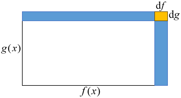
First, place the function $h(x)=f(x) \cdot g(x)$ in the example of finding the area of a rectangle: $h(x)$ is the area of the rectangle, $f(x)$ is the width, and $g(x)$ is the height. When the variable $x$ changes by a tiny amount, the differential interpretation says this represents the rate of change of the rectangle’s area, as shown below.
-
Here, $\mathrm{d} h$ is the change in area, namely the blue part in the figure: $\mathrm{d} h=\mathrm{d} f \cdot g(x)+f(x) \cdot \mathrm{d} g+\mathrm{d} f \cdot \mathrm{d} g$,
-
Since $\mathrm{d} f \cdot \mathrm{d} g$ is a second-order infinitesimal, it is approximately 0 and can be neglected;
-
Dividing both sides of the equation by $\mathrm{d} x$ gives the product rule $\frac{\mathrm{d} h}{\mathrm{~d} x}=\frac{\mathrm{d} f}{\mathrm{~d} x} g(x)+f(x) \frac{\mathrm{d} g}{\mathrm{~d} x}$.
-
At this point, $\mathrm{d} h$ is the change in area, while $\frac{\mathrm{d} h}{\mathrm{~d} x}$ is the rate of change of the area.
Similarly, we can continue and derive the power rule for derivatives:
$$
\frac{\mathrm{d}\left(x^n\right)}{\mathrm{d} x}=n x^{n-1}$$
Using the same example, if both $f(x)$ and $g(x)$ are equal to $x$, then $h(x)=x^2, \mathrm{~d} h=\mathrm{d} x^2$, as shown below.

The change in the area of the square is derived as follows:
$$
\mathrm{d} h=x \cdot \mathrm{d} x+x \cdot \mathrm{d} x+\mathrm{d} x \cdot \mathrm{d} x=2 x \mathrm{~d} x$$
Because $\mathrm{d} h=\mathrm{d} x^2$, substituting and rearranging gives $\frac{\mathrm{d} x^2}{\mathrm{~d} x}=2 x$.
This derived result is consistent with the result obtained directly using the power rule, $\mathrm{d} h=\mathrm{d} x^2=2 x$.
The same method extends to three-dimensional space, and the derivations of the product rule and power rule still apply, as shown in the figure:
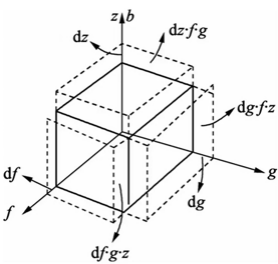
Here the volume is $y=f(x) \cdot g(x) \cdot z(x)$, and the change in volume is:
$$
\mathrm{d} y=\mathrm{d} f \cdot g \cdot z+\mathrm{d} g \cdot f \cdot z+\mathrm{d} z \cdot f \cdot g$$
If $f(x)$, $g(x)$, and $z(x)$ are all equal to $x$, then the change in volume $\mathrm{d} y$ is:
$$
\begin{aligned}
\mathrm{d} y & =\mathrm{d} x \cdot x^2+\mathrm{d} x \cdot x^2+\mathrm{d} x \cdot x^2 \\
& =3 x^2 \mathrm{~d} x \\
\end{aligned}$$
The rate of change of the volume, $\frac{\mathrm{d} y}{\mathrm{~d} x}$, is:
$$
\frac{\mathrm{d} y}{\mathrm{~d} x}=3 x^2$$
You can imagine that this continues to apply in higher-dimensional spaces, although it is no longer convenient to visualize here.
Differentiation and Monotonicity of Functions
Let’s start directly with the definition:
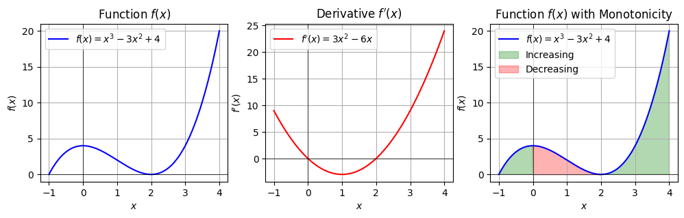
- If $f(x)$ is differentiable on $(a, b)$ and $f^{\prime}(x)>0$, then the function is monotonically increasing on $(a, b)$;
- If $f^{\prime}(x)<0$, then the function is monotonically decreasing on $(\mathrm{a}, \mathrm{b})$.
The definition of the differential—that it explains the pattern of change of a function—also makes monotonicity easy to interpret. When a change in $x$ causes the function to increase, the function is monotonically increasing. When a change in $x$ causes the function to decrease, the function is monotonically decreasing.
import numpy as np
import matplotlib.pyplot as plt

# Define the function f(x)
def f(x):
    return x**3 - 3*x**2 + 4

# Define the derivative f'(x)
def df(x):
    return 3*x**2 - 6*x

# Create points on the x-axis
x = np.linspace(-1, 4, 400)

# Compute function and derivative values
y = f(x)
dy = df(x)

# Plot the function f(x) and its derivative f'(x)
plt.figure(figsize=(12, 3))

# Plot f(x)
plt.subplot(1, 3, 1)
plt.plot(x, y, label='$f(x) = x^3 - 3x^2 + 4$', color='b')
plt.title('Function $f(x)$')
plt.xlabel('$x$')
plt.ylabel('$f(x)$')
plt.axhline(0, color='black',linewidth=0.5)
plt.axvline(0, color='black',linewidth=0.5)
plt.grid(True)
plt.legend()

# Plot f'(x)
plt.subplot(1, 3, 2)
plt.plot(x, dy, label="$f'(x) = 3x^2 - 6x$", color='r')
plt.title('Derivative $f'(x)$')
plt.xlabel('$x$')
plt.ylabel("$f'(x)$")
plt.axhline(0, color='black',linewidth=0.5)
plt.axvline(0, color='black',linewidth=0.5)
plt.grid(True)
plt.legend()

# Plot f(x)
plt.subplot(1, 3, 3)
plt.plot(x, y, label='$f(x) = x^3 - 3x^2 + 4$', color='b')
plt.fill_between(x, y, where=(dy > 0), interpolate=True, color='green', alpha=0.3, label='Increasing')
plt.fill_between(x, y, where=(dy < 0), interpolate=True, color='red', alpha=0.3, label='Decreasing')
plt.title('Function $f(x)$ with Monotonicity')
plt.xlabel('$x$')
plt.ylabel('$f(x)$')
plt.axhline(0, color='black',linewidth=0.5)
plt.axvline(0, color='black',linewidth=0.5)
plt.grid(True)
plt.legend()

plt.show()
Extrema and Saddle Points
- Extrema:
- Local Maximum: at a point $x=a$, if the function value $f(a)$ is greater than the function values at all other points in its neighborhood, then $f(a)$ is a local maximum.
- Local Minimum: at a point $x=b$, if the function value $f(b)$ is less than the function values at all other points in its neighborhood, then $f(b)$ is a local minimum.
- Saddle Point:
- A saddle point is a point $x=c$ where the derivative of the function is zero, but the point is neither a local maximum nor a local minimum.
import numpy as np
import matplotlib.pyplot as plt
from sympy import symbols, diff, solve
from mpl_toolkits.mplot3d import Axes3D

# Define symbolic variables and the function
x, y = symbols('x y')
f_sym = x**3 - 3*x + y**3 - 3*y
df_sym_x = diff(f_sym, x)
df_sym_y = diff(f_sym, y)

# Solve for points where the first derivative is zero (critical points)
critical_points = solve((df_sym_x, df_sym_y), (x, y))

# Compute the second derivative and evaluate the nature of the critical points
d2f_sym_xx = diff(df_sym_x, x)
d2f_sym_yy = diff(df_sym_y, y)
d2f_sym_xy = diff(df_sym_x, y)

# Visualization
x_vals = np.linspace(-3, 3, 100)
y_vals = np.linspace(-3, 3, 100)
x_vals, y_vals = np.meshgrid(x_vals, y_vals)
f_vals = x_vals**3 - 3*x_vals + y_vals**3 - 3*y_vals

fig = plt.figure(figsize=(14, 8))
ax = fig.add_subplot(111, projection='3d')

# Plot the function f(x, y)
ax.plot_surface(x_vals, y_vals, f_vals, cmap='viridis', alpha=0.7)

# Mark the critical points and their nature
for point in critical_points:
    x_val, y_val = float(point[0]), float(point[1])
    z_val = x_val**3 - 3*x_val + y_val**3 - 3*y_val
    d2f_xx_val = d2f_sym_xx.subs({x: x_val, y: y_val})
    d2f_yy_val = d2f_sym_yy.subs({x: x_val, y: y_val})

    if d2f_xx_val > 0 and d2f_yy_val > 0:
        ax.scatter(x_val, y_val, z_val, color='g', s=100, label='Local Min' if 'Local Min' not in ax.get_legend_handles_labels()[1] else "")
    elif d2f_xx_val < 0 and d2f_yy_val < 0:
        ax.scatter(x_val, y_val, z_val, color='r', s=100, label='Local Max' if 'Local Max' not in ax.get_legend_handles_labels()[1] else "")
    else:
        ax.scatter(x_val, y_val, z_val, color='y', s=100, label='Saddle Point' if 'Saddle Point' not in ax.get_legend_handles_labels()[1] else "")

ax.set_title('3D Visualization of $f(x, y) = x^3 - 3x + y^3 - 3y$')
ax.set_xlabel('$x$')
ax.set_ylabel('$y$')
ax.set_zlabel('$f(x, y)$')
ax.legend()
plt.show()
Hessian Matrix
The Hessian matrix is a square matrix used to describe the local second-order behavior of a multivariable function at a point. For an $n$-dimensional function $f(\mathbf{x})$, where $\mathbf{x}=\left(x_1, x_2, \ldots, x_n\right)$, the Hessian matrix $H$ is defined as:
$$
H(\mathbf{x})=\left(\begin{array}{cccc}
\frac{\partial^2 f}{\partial x_1^2} & \frac{\partial^2 f}{\partial x_1 \partial x_2} & \cdots & \frac{\partial^2 f}{\partial x_1 \partial x_n} \\
\frac{\partial^2 f}{\partial x_2 \partial x_1} & \frac{\partial^2 f}{\partial x_2^2} & \cdots & \frac{\partial^2 f}{\partial x_2 \partial x_n} \\
\vdots & \vdots & \ddots & \vdots \\
\frac{\partial^2 f}{\partial x_n \partial x_1} & \frac{\partial^2 f}{\partial x_n \partial x_2} & \cdots & \frac{\partial^2 f}{\partial x_n^2} \\
\end{array}\right)$$
Here, $\frac{\partial^2 f}{\partial x_i \partial x_j}$ denotes the second partial derivative of $f$ with respect to $x_i$ and $x_j$.
The Hessian matrix is mainly used to analyze the nature of critical points of multivariable functions—that is, to determine whether these points are local extrema (maxima or minima) or saddle points. The specific steps are as follows:
-
Find the critical points: solve for the points where the first-order partial derivatives are zero.
$$
\nabla f(\mathbf{x})=\left(\frac{\partial f}{\partial x_1}, \frac{\partial f}{\partial x_2}, \ldots, \frac{\partial f}{\partial x_n}\right)=0$$ -
Compute the Hessian matrix: evaluate the Hessian matrix $H$ at each critical point.
-
Discriminant method:
- Compute the determinant $D$: compute the determinant and eigenvalues of the Hessian matrix to determine the nature of the critical point.
- For a two-variable function $f(x, y)$, the determinant $D$ is computed as follows:
$$
D=\operatorname{det}(H)=f_{x x} f_{y y}-\left(f_{x y}\right)^2$$
- Determine the nature of the critical point:
- If D>0, it is an extremum.
- If D<0, it is a saddle point.
- If D=0, further analysis is needed (the nature is usually indeterminate).
The determinant D is only a tool for helping distinguish extrema from saddle points. To determine the nature of a critical point accurately (maximum or minimum), eigenvalues are needed. The specific criteria are:
- If all eigenvalues are positive, the function has a local minimum at that point.
- If all eigenvalues are negative, the function has a local maximum at that point.
- If the eigenvalues include both positive and negative values, the function has a saddle point at that point.
- If any eigenvalue is zero, further analysis is needed (the nature is usually indeterminate).
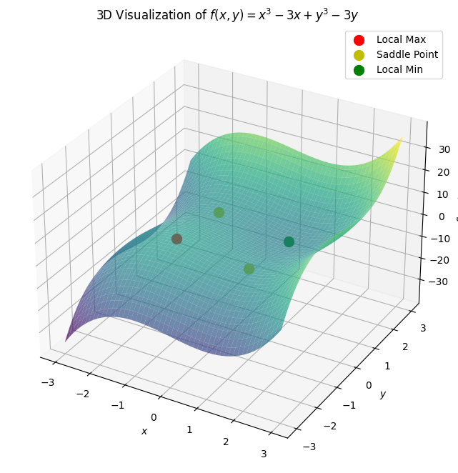
For example, the analysis of the function $f(x, y)=x^3-3 x+y^3-3 y$ is as follows:
-
First, find the critical points:
$$
\begin{aligned}
& f_x=3 x^2-3=0 \Longrightarrow x= \pm 1 \\
& f_y=3 y^2-3=0 \Longrightarrow y= \pm 1 \\
\end{aligned}$$ -
Then compute the Hessian matrix:
$$
H=\left(\begin{array}{cc}
6 x & 0 \\
0 & 6 y \\
\end{array}\right)$$
- The characteristic equation is:
$$
\operatorname{det}\left(\begin{array}{cc}
6 x-\lambda & 0 \\
0 & 6 y-\lambda \\
\end{array}\right)=0$$
Solving gives the eigenvalues $\lambda_1=6 x$ and $\lambda_2=6 y$.
At the critical point $(1,1)$:
- Eigenvalue $\lambda_1=6 \cdot 1=6>0$
- Eigenvalue $\lambda_2=6 \cdot 1=6>0$
Therefore, $(1,1)$ is a local minimum.
At the critical point $(1,-1)$:
- Eigenvalue $\lambda_1=6 \cdot 1=6>0$
- Eigenvalue $\lambda_2=6 \cdot(-1)=-6<0$
Therefore, $(1,-1)$ is a saddle point. The nature of the other critical points can be analyzed in the same way.
Concavity and Convexity of Functions
- Concavity and convexity describe the shape of a function. More specifically, they tell us whether the curve bends upward or downward.
- Convex Function: geometrically, this means that the line segment connecting any two points on the curve lies above the curve or coincides with it.
- Concave Function: geometrically, this means that the line segment connecting any two points on the curve lies below the curve or coincides with it.
The Hessian matrix can be used to determine the concavity or convexity of a function.
- If all eigenvalues are positive, the Hessian matrix is positive definite, and the function is convex near that point.
- If all eigenvalues are negative, the Hessian matrix is negative definite, and the function is concave near that point.
- If the eigenvalues include both positive and negative values, the function is neither convex nor concave near that point.
 The Chain Rule
In machine learning, especially in deep learning and neural networks, the chain rule is used to compute derivatives of composite functions, which is particularly important in the backpropagation algorithm. More specifically, when training a deep neural network, we need to compute the gradient of the loss function with respect to each weight. Because each layer of a neural network is composite, the chain rule lets us work backward step by step from the output layer to the input layer to compute these gradients.
First, let’s look at the mathematical formula for the differential chain rule:
$$
\begin{gathered}
y=f(g(x))
\frac{\mathrm{d} y}{\mathrm{~d} x}=\frac{\mathrm{d} f}{\mathrm{~d} x}=\frac{\mathrm{d} f}{\mathrm{~d} g} \cdot \frac{\mathrm{d} g}{\mathrm{~d} x}=f^{\prime}(g(x)) \cdot \mathrm{g}^{\prime}(x)
\end{gathered}$$
The idea is simple: like peeling an onion, we uncover the inner core layer by layer. The chain rule is generally used to differentiate composite functions: first differentiate the outer function, then multiply by the derivative of the inner function. We have repeatedly emphasized that the derivative describes the pattern of change of a function, so the chain rule is the rule by which changes are transmitted.
Example:
$$
\begin{aligned}
& y=\sin \left(x^2\right) \\
& h=x^2 \\
& y=\sin (h) \\
\end{aligned}$$
The steps for differentiating $y$ are as follows:
$$
\begin{aligned}
& \frac{\mathrm{d} y}{\mathrm{~d} h}=\cos h \quad \mathrm{~d} y=\cos h \mathrm{~d} h \\
& \mathrm{~d} h=\mathrm{d} x^2=2 x \mathrm{~d} x \\
& \mathrm{~d} y=\cos x^2 \cdot 2 x \mathrm{~d} x \Rightarrow \frac{\mathrm{d} y}{\mathrm{~d} x}=\cos x^2 \cdot 2 x \\
\end{aligned}$$
To explain: a change in $x$ causes a change in $h$, which in turn causes a change in $y$. The chain rule is the rule of how changes are transmitted.
Gradient
- Mathematical definition of the gradient
For a multivariable scalar function $f\left(x_1, x_2, \ldots, x_n\right)$, the gradient is a vector composed of partial derivatives. The gradient vector represents the rate of change of $f$ in each direction. Mathematically, the gradient can be written as:
$$
\nabla f=\left(\frac{\partial f}{\partial x_1}, \frac{\partial f}{\partial x_2}, \ldots, \frac{\partial f}{\partial x_n}\right)$$
Here, $\frac{\partial f}{\partial x_i}$ denotes the partial derivative of $f$ with respect to the $i$-th variable $x_i$.
- Geometric interpretation of the gradient
The gradient vector points in the direction in which the function value increases fastest, and its magnitude equals the maximum rate of change in that direction. For example, in the two-dimensional plane, if we have a scalar function $f(x, y)$, its gradient is:
$$
\nabla f=\left(\frac{\partial f}{\partial x}, \frac{\partial f}{\partial y}\right)$$
At this point, the gradient vector $\nabla f$ points in the direction in which $f$ increases fastest, and its length represents the maximum rate of change of $f$ in that direction.
- Applications of the gradient in deep learning
Gradient descent is a commonly used optimization algorithm. By moving in the opposite direction of the gradient, it gradually approaches the minimum of a function. Gradient descent is widely used for parameter optimization in machine learning.
- Example of gradient calculation
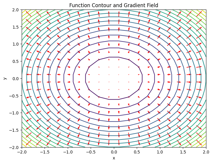
Consider a simple two-dimensional function $f(x, y)=x^2+y^2$. We can compute its gradient:
$$
\nabla f=\left(\frac{\partial f}{\partial x}, \frac{\partial f}{\partial y}\right)=(2 x, 2 y)$$
This shows that at any point $(x, y)$, the gradient vector $(2 x, 2 y)$ points in the direction in which the function value increases fastest, and its magnitude is $\sqrt{(2 x)^2+(2 y)^2}=2 \sqrt{x^2+y^2}$. Next, let’s further understand the concept of the gradient by plotting a contour map (level-curve plot) of a function together with its gradient field.
import numpy as np
import matplotlib.pyplot as plt

# Define the function
def f(x, y):
    return x**2 + y**2

# Define the gradient function
def gradient_f(x, y):
    return np.array([2*x, 2*y])

# Create the grid
x = np.linspace(-2, 2, 20)
y = np.linspace(-2, 2, 20)
X, Y = np.meshgrid(x, y)
Z = f(X, Y)

# Compute the gradient
U, V = gradient_f(X, Y)

# Plot the contour map and gradient field
plt.figure(figsize=(8, 6))
plt.contour(X, Y, Z, levels=20)
plt.quiver(X, Y, U, V, color='r')

plt.title('Function Contour and Gradient Field')
plt.xlabel('x')
plt.ylabel('y')
plt.show()
 Taylor Series
Taylor’s formula allows complex functions to be approximated by polynomials, which is sometimes used in algorithms to simplify computation. For example, in Gaussian process regression and some other Bayesian methods, Taylor expansion is used to linearize computations related to the posterior.
The essence of Taylor’s formula is to use simple polynomials to approximate and fit complex functions.
First, recall differentiation:
$$
\frac{f\left(x_0+\Delta x\right)-f\left(x_0\right)}{\Delta x} \approx f^{\prime}\left(x_0\right)$$
If $f^{\prime}\left(x_0\right)$ exists, then near $x_0$ we have $f\left(x_0+\Delta x\right)-f\left(x_0\right) \approx f^{\prime}\left(x_0\right) \Delta x$. Let $\Delta x=x-x_0$; substituting $\Delta x$ into the expression above and rearranging gives:
$$
f(x) \approx f\left(x_0\right)+f^{\prime}\left(x_0\right)\left(x-x_0\right)$$
This is the origin of the idea behind Taylor’s formula: the function $f(x)$ may be very complex, perhaps even too complex to write down explicitly, but it can be approximated using the function value $f\left(x_0\right)$ at a point $\mathrm{P}$ and the derivative $f^{\prime}\left(x_0\right)$ at that point. To explain further: first, we want the approximating function to pass through the given point, such as the value $f\left(x_0\right)$ at point $\mathrm{P}$. Then, to ensure that the shape of the approximating function is similar to the original function, we want their slopes at point $\mathrm{P}$ to be the same. This is why the first derivative is used.
However, knowing only the slope at point P may not be enough to describe the entire shape of the function. To model the shape more accurately, we may need to consider the degree of curvature, namely concavity or convexity. This is why the second derivative is considered. Then, to capture more details, we may need third-, fourth-, or even higher-order derivatives. The more derivative orders we use, the stronger the constraints on the function, and the more precisely we can fit a definite function. Therefore, Taylor’s formula can be written as:
$$
P_n(x)=f\left(x_0\right)+f^{\prime}\left(x_0\right)\left(x-x_0\right)+\frac{f^{\prime \prime}\left(x_0\right)}{2!}\left(x-x_0\right)^2+\cdots+\frac{f^{(n)}\left(x_0\right)}{n!}\left(x-x_0\right)^n$$
We have just introduced derivative order. Now let’s think about what the polynomial term $\left(x-x_0\right)^n, n=1,2,3 \cdots$ is used for.
Compute the Taylor polynomials of different orders for $f(x)=e^x$ at the point $x=0$, as in the following code:
import numpy as np
import matplotlib.pyplot as plt

# Define the original function and Taylor expansion terms
def f(x):
    return np.exp(x)

def taylor_approx(x, n):
    result = 0
    for i in range(n + 1):
        result += (x**i) / np.math.factorial(i)
    return result

# Generate data points
x = np.linspace(-2, 2, 400)
y = f(x)

# Create a figure with a 2x2 grid of subplots
fig, axs = plt.subplots(2, 2, figsize=(6, 6))

# Plot Taylor polynomial approximations of different orders
for n, ax in zip(range(1, 5), axs.ravel()):
    ax.plot(x, y, label='$e^x$', color='black')
    ax.plot(x, taylor_approx(x, n), label=f'Taylor Polynomial (n={n})')
    ax.set_title(f'Taylor Series Approximation of $e^x$ at $x=0$, n={n}')
    ax.set_xlabel('x')
    ax.set_ylabel('y')
    ax.legend()
    ax.grid(True)

# Adjust the layout to prevent label overlap
plt.tight_layout()
plt.show()
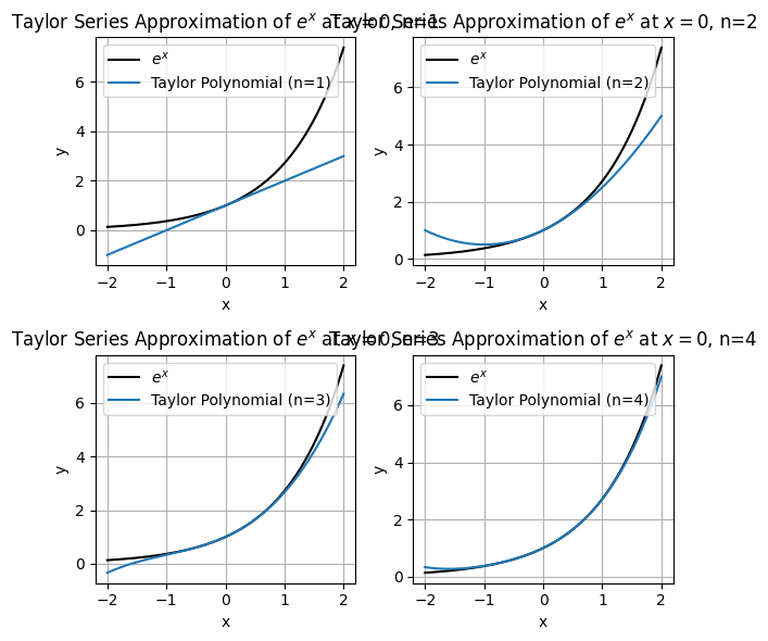
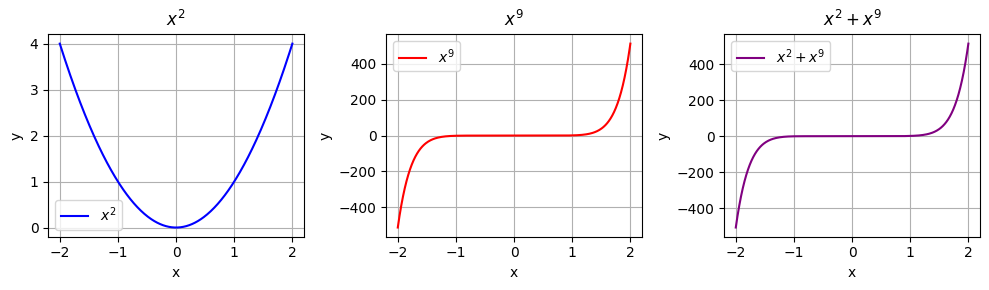
Imagine using a curve to approximate the shape of a mountain (a complex function). If we use only a straight line (a linear function), it may describe only one slope of the mountain roughly. But if we use a curve, such as a quadratic or higher-degree function, we can describe the mountain’s outline more accurately. In other words, low-order terms (such as linear or quadratic terms) usually dominate near the starting part of the function, while high-order terms (such as cubic, quartic, or higher terms) dominate farther away. This is why Taylor’s formula contains polynomial terms. Finally, let’s explain the role of the factorial $n!$. As shown below, consider $x^2$ and $x^9$. When $x$ is large, $x^2$ is completely dominated by $x^9$, and $x^9+x^2$ almost only exhibits the behavior of $x^9$. Therefore, because higher-order power functions grow too quickly, we divide by the factorial to slow down the growth.
import numpy as np
import matplotlib.pyplot as plt

# Generate data points
x = np.linspace(-2, 2, 400)

# Define the power functions
y_x2 = x**2
y_x9 = x**9
y_sum = x**2 + x**9

# Create a figure with a 3x1 grid of subplots
fig, axs = plt.subplots(1, 3, figsize=(10, 3))

# Plot the $x^2$ curve
axs[0].plot(x, y_x2, label='$x^2$', color='blue')
axs[0].set_title('$x^2$')
axs[0].set_xlabel('x')
axs[0].set_ylabel('y')
axs[0].legend()
axs[0].grid(True)

# Plot the $x^9$ curve
axs[1].plot(x, y_x9, label='$x^9$', color='red')
axs[1].set_title('$x^9$')
axs[1].set_xlabel('x')
axs[1].set_ylabel('y')
axs[1].legend()
axs[1].grid(True)

# Plot the $x^2 + x^9$ curve
axs[2].plot(x, y_sum, label='$x^2 + x^9$', color='purple')
axs[2].set_title('$x^2 + x^9$')
axs[2].set_xlabel('x')
axs[2].set_ylabel('y')
axs[2].legend()
axs[2].grid(True)

# Adjust the layout to prevent label overlap
plt.tight_layout()
plt.show()
Finally, to restate the essence of Taylor’s formula: when a complex function is too difficult to solve directly, it can be fitted using the value of the function at a point and the higher-order derivatives at that point.
 Fourier series
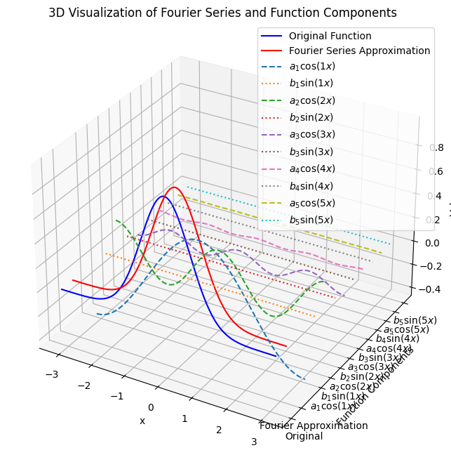
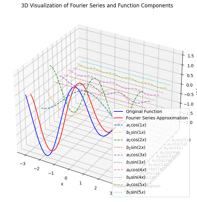
- A Fourier series is a method for representing a periodic function as an infinite series of trigonometric functions (sine and cosine functions). It was proposed by the French mathematician Joseph Fourier and is widely used in many areas of mathematics and engineering.
- The basic idea of a Fourier series is to decompose a periodic function into a sum of sine and cosine functions with different frequencies.
For a function $f(x)$ with period $2 \pi$, it can be represented as:
$$
f(x)=\frac{a_0}{2}+\sum_{n=1}^{\infty}\left(a_n \cos (n x)+b_n \sin (n x)\right)$$
where:
- $a_0$ is the average value of the function (the DC component), computed by:
$$
a_0=\frac{1}{\pi} \int_{-\pi}^\pi f(x) d x$$
- $a_n$ and $b_n$ are Fourier coefficients, representing the coefficients of the cosine and sine terms respectively, computed as:
$$
\begin{aligned}
& a_n=\frac{1}{\pi} \int_{-\pi}^\pi f(x) \cos (n x) d x \\
& b_n=\frac{1}{\pi} \int_{-\pi}^\pi f(x) \sin (n x) d x \\
\end{aligned}$$
These coefficients $a_n$ and $b_n$ describe the amplitudes of the sine and cosine components of the function at different frequencies.
import numpy as np
import matplotlib.pyplot as plt
from mpl_toolkits.mplot3d import Axes3D

# Define the function f(x)
def f(x):
    return np.sin(x) + 0.5 * np.cos(2 * x) +np.cos(1.5 * x) # Example function, you can change this to any 2π periodic function

# Number of terms in the Fourier series
N = 5

# Calculate Fourier coefficients
a0 = (1 / np.pi) * np.trapz(f(np.linspace(-np.pi, np.pi, 1000)), np.linspace(-np.pi, np.pi, 1000))
an = [(1 / np.pi) * np.trapz(f(np.linspace(-np.pi, np.pi, 1000)) * np.cos(n * np.linspace(-np.pi, np.pi, 1000)), np.linspace(-np.pi, np.pi, 1000)) for n in range(1, N+1)]
bn = [(1 / np.pi) * np.trapz(f(np.linspace(-np.pi, np.pi, 1000)) * np.sin(n * np.linspace(-np.pi, np.pi, 1000)), np.linspace(-np.pi, np.pi, 1000)) for n in range(1, N+1)]

# Create the Fourier series approximation
def fourier_series(x, a0, an, bn, N):
    result = a0 / 2
    for n in range(1, N+1):
        result += an[n-1] * np.cos(n * x) + bn[n-1] * np.sin(n * x)
    return result

# Prepare the data
x = np.linspace(-np.pi, np.pi, 1000)
y_original = f(x)
y_approx = fourier_series(x, a0, an, bn, N)

# Create a figure for 3D plotting
fig = plt.figure(figsize=(14, 8))
ax = fig.add_subplot(111, projection='3d')

# Plot the original function
ax.plot(x, y_original, zs=0, zdir='y', label='Original Function', color='b')

# Plot the Fourier series approximation
ax.plot(x, y_approx, zs=1, zdir='y', label='Fourier Series Approximation', color='r')

# Plot individual sine and cosine components
for n in range(1, N+1):
    ax.plot(x, an[n-1] * np.cos(n * x), zs=2 + 2 * n - 1, zdir='y', label=f'$a_{n} cos({n}x)$', linestyle='dashed')
    ax.plot(x, bn[n-1] * np.sin(n * x), zs=2 + 2 * n, zdir='y', label=f'$b_{n} sin({n}x)$', linestyle='dotted')

# Set labels and title
ax.set_xlabel('x')
ax.set_ylabel('Function Components')
ax.set_zlabel('Value')
ax.set_title('3D Visualization of Fourier Series and Function Components')

# Set yticks to show labels clearly
yticks = [0, 1] + [2 + 2 * n - 1 for n in range(1, N+1)] + [2 + 2 * n for n in range(1, N+1)]
ytick_labels = ['Original', 'Fourier Approximation'] + [f'$a_{n} cos({n}x)$' for n in range(1, N+1)] + [f'$b_{n} sin({n}x)$' for n in range(1, N+1)]
ax.set_yticks(yticks)
ax.set_yticklabels(ytick_labels)

ax.legend()
plt.show()
For non-periodic functions, the usual approaches are:
- Truncation: truncate the non-periodic function on a finite interval so that it is approximately periodic on that interval. The truncated function can then be approximated by a Fourier series on the finite interval.
- Fourier transform: use the Fourier transform to analyze the function’s spectrum and find its representation in the frequency domain. The Fourier transform can represent any function as a linear combination of sine and cosine functions.
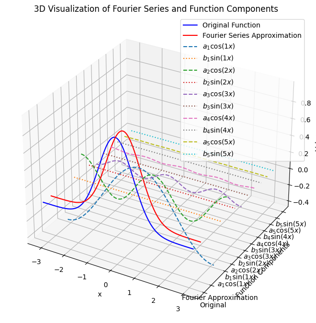
import numpy as np
import matplotlib.pyplot as plt
from mpl_toolkits.mplot3d import Axes3D

# Define the function f(x)
def f(x):
    return np.exp(-x**2)  # Example non-periodic function, Gaussian

# Number of terms in the Fourier series
N = 5

# Calculate Fourier coefficients
a0 = (1 / np.pi) * np.trapz(f(np.linspace(-np.pi, np.pi, 1000)), np.linspace(-np.pi, np.pi, 1000))
an = [(1 / np.pi) * np.trapz(f(np.linspace(-np.pi, np.pi, 1000)) * np.cos(n * np.linspace(-np.pi, np.pi, 1000)), np.linspace(-np.pi, np.pi, 1000)) for n in range(1, N+1)]
bn = [(1 / np.pi) * np.trapz(f(np.linspace(-np.pi, np.pi, 1000)) * np.sin(n * np.linspace(-np.pi, np.pi, 1000)), np.linspace(-np.pi, np.pi, 1000)) for n in range(1, N+1)]

# Create the Fourier series approximation
def fourier_series(x, a0, an, bn, N):
    result = a0 / 2
    for n in range(1, N+1):
        result += an[n-1] * np.cos(n * x) + bn[n-1] * np.sin(n * x)
    return result

# Prepare the data
x = np.linspace(-np.pi, np.pi, 1000)
y_original = f(x)
y_approx = fourier_series(x, a0, an, bn, N)

# Create a figure for 3D plotting
fig = plt.figure(figsize=(14, 8))
ax = fig.add_subplot(111, projection='3d')

# Plot the original function
ax.plot(x, y_original, zs=0, zdir='y', label='Original Function', color='b')

# Plot the Fourier series approximation
ax.plot(x, y_approx, zs=1, zdir='y', label='Fourier Series Approximation', color='r')

# Plot individual sine and cosine components
for n in range(1, N+1):
    ax.plot(x, an[n-1] * np.cos(n * x), zs=2 + 2 * n - 1, zdir='y', label=f'$a_{n} cos({n}x)$', linestyle='dashed')
    ax.plot(x, bn[n-1] * np.sin(n * x), zs=2 + 2 * n, zdir='y', label=f'$b_{n} sin({n}x)$', linestyle='dotted')

# Set labels and title
ax.set_xlabel('x')
ax.set_ylabel('Function Components')
ax.set_zlabel('Value')
ax.set_title('3D Visualization of Fourier Series and Function Components')

# Set yticks to show labels clearly
yticks = [0, 1] + [2 + 2 * n - 1 for n in range(1, N+1)] + [2 + 2 * n for n in range(1, N+1)]
ytick_labels = ['Original', 'Fourier Approximation'] + [f'$a_{n} cos({n}x)$' for n in range(1, N+1)] + [f'$b_{n} sin({n}x)$' for n in range(1, N+1)]
ax.set_yticks(yticks)
ax.set_yticklabels(ytick_labels)

ax.legend()
plt.show()
 Credits
- Icons made by Becris from www.flaticon.com
- Icons from Icons8.com – https://icons8.com
- Datasets from Kaggle – https://www.kaggle.com/
- Introduction to AutoDiff by Alexey Radul
- Gentle Introduction to AutoDiff by Boris Ettinger
- Statistical Machine Learning – Automatic Differentiation and Neural Networks – Jason Domke
- AUTOGRAD: AUTOMATIC DIFFERENTIATION
Tal Daniel