Learning Methods of Deep Learning

Created by Deepfinder

Agenda

1. Learning from a Teacher: Supervised Learning
2. Seeing the Big Picture from Small Clues: Unsupervised Learning
3. Learning without a Teacher: Self-supervised Learning
4. From a Few Points to the Whole: Semi-supervised Learning
5. Distinguishing Right from Wrong: Contrastive Learning
6. Learning by Analogy: Transfer Learning
7. Head-to-Head: Adversarial Learning
8. United We Stand: Ensemble Learning
9. Different Paths to the Same Goal: Federated Learning
10. Persevering through Trials: Reinforcement Learning
11. Eager to Learn: Active Learning
12. Learning to Learn: Meta-Learning

Tutorial 02 – Seeing the Big Picture from Small Clues: Unsupervised Learning

Auto-encoders

• Most natural data is high-dimensional, such as images. Consider the MNIST handwritten digit dataset. Each image has $28×28=784$ pixels, so it can be represented as a vector of length 784.
• But do we really need 784 values to represent one digit? The answer is no. We assume that the data lies in a low-dimensional space that is enough to describe the observations. In the MNIST case, we can choose to represent digits as one-hot vectors, which means we only need 10 dimensions. Therefore, we can encode high-dimensional observations in a low-dimensional space.

But how can we learn meaningful low-dimensional representations?

The general idea is to reconstruct, or decode, the low-dimensional representation back into a high-dimensional representation. We then use the reconstruction error to find the best representation, by using the gradient of the error. This is the core idea behind auto-encoders.

• Auto-encoder – A model that takes data as input and discovers a latent state representation of that data. The input data is converted into an encoded vector. Each dimension represents a learned property of the data. The most important detail here is that the encoder network outputs one value for each encoded dimension. Then the decoder network takes these values and tries to recreate the original input.
• An auto-encoder has three parts: an encoder, a decoder, and a “loss” function that maps one part to the other. For the simplest auto-encoder, which compresses the input and then reconstructs the original input from the compressed representation, we can view the “loss” as the amount of information lost during reconstruction.

Image Source

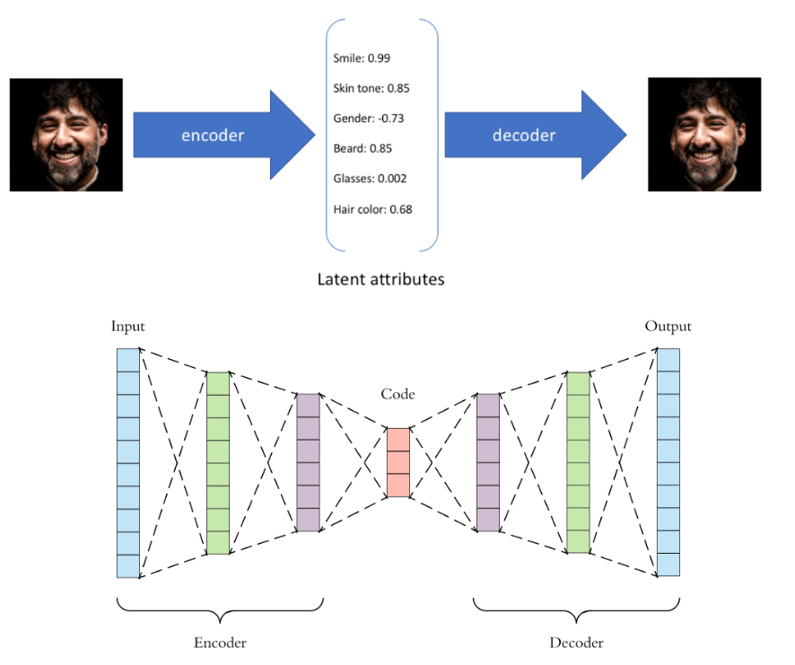
Let’s implement it in PyTorch using what we have learnt so far!

import torch
import torch.nn as nn 
import torchvision 
import matplotlib.pyplot as plt
import time
# Fashion-MNIST
fmnist_train_dataset = torchvision.datasets.FashionMNIST(root='./datasets/',
                                           train=True, 
                                           transform=torchvision.transforms.ToTensor(),
                                           download=True)

fmnist_test_dataset = torchvision.datasets.FashionMNIST(root='./datasets',
                                          train=False, 
                                          transform=torchvision.transforms.ToTensor())

# Data loader
fmnist_train_loader = torch.utils.data.DataLoader(dataset=fmnist_train_dataset,
                                           batch_size=64, 
                                           shuffle=True, drop_last=True)

fmnist_test_loader = torch.utils.data.DataLoader(dataset=fmnist_test_dataset,
                                          batch_size=64, 
                                          shuffle=False)

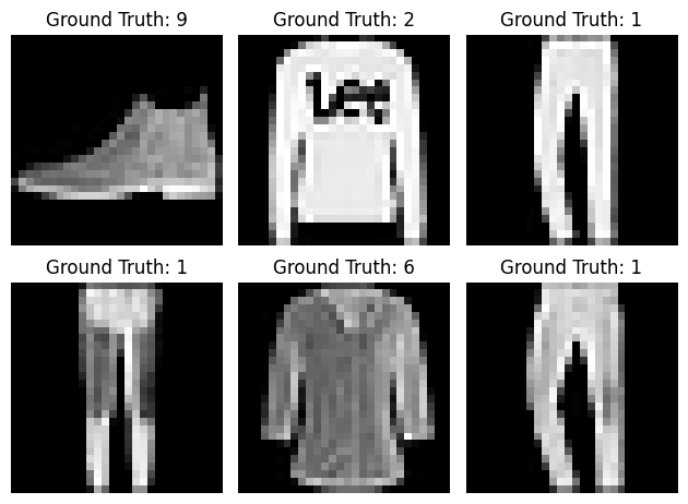
# let's plot some of the samples from the test set
examples = enumerate(fmnist_test_loader)
batch_idx, (example_data, example_targets) = next(examples)
print("shape: \n", example_data.shape)
fig = plt.figure()
for i in range(6):
    ax = fig.add_subplot(2,3,i+1)
    ax.imshow(example_data[i][0], cmap='gray', interpolation='none')
    ax.set_title("Ground Truth: {}".format(example_targets[i]))
    ax.set_axis_off()
plt.tight_layout()

shape: 
 torch.Size([64, 1, 28, 28])

class AutoEncoder(nn.Module):

    def __init__(self, input_dim=28*28, hidden_dim=256, latent_dim=10):
        super(AutoEncoder, self).__init__()

        self.input_dim = input_dim
        self.hidden_dim = hidden_dim
        self.latent_dim = latent_dim

        # define the encoder
        self.encoder = nn.Sequential(nn.Linear(self.input_dim, self.hidden_dim),
                                     nn.ReLU(), 
                                     nn.Linear(self.hidden_dim, self.hidden_dim),
                                     nn.ReLU(),
                                     nn.Linear(self.hidden_dim, self.latent_dim)
                                    )

        # define decoder
        self.decoder = nn.Sequential(nn.Linear(self.latent_dim, self.hidden_dim),
                                     nn.ReLU(),
                                     nn.Linear(self.hidden_dim, self.hidden_dim),
                                     nn.ReLU(),
                                     nn.Linear(self.hidden_dim, self.input_dim),
                                     nn.Sigmoid())

    def forward(self,x):
        x = self.encoder(x)
        x = self.decoder(x)
        return x

    def get_latent_rep(self, x):
        return self.encoder(x)

# hyper-parameters:
num_epochs = 5
learning_rate = 0.001

# Device configuration, as before
device = torch.device('cuda:0' if torch.cuda.is_available() else 'cpu')

# create model, send it to device
model = AutoEncoder(input_dim=28 * 28, hidden_dim=128, latent_dim=10).to(device)

# Loss and optimizer
criterion = nn.BCELoss()  # binary cross entropy, as pixels are in [0,1]
optimizer = torch.optim.Adam(model.parameters(), lr=learning_rate)

# Train the model
total_step = len(fmnist_train_loader)
start_time = time.time()
for epoch in range(num_epochs):
    for i, (images, labels) in enumerate(fmnist_train_loader): 
        images = images.to(device).view(64, -1)

        # Forward pass
        outputs = model(images)
        loss = criterion(outputs, images)

        # Backward and optimize - ALWAYS IN THIS ORDER!
        optimizer.zero_grad()
        loss.backward()
        optimizer.step()

        if (i + 1) % 100 == 0:
            print ('Epoch [{}/{}], Step [{}/{}], Loss: {:.4f}, Time: {:.4f} secs' 
                   .format(epoch + 1, num_epochs, i + 1, total_step, loss.item(), time.time() - start_time))

Epoch [1/5], Step [100/937], Loss: 0.3769, Time: 0.4937 secs
Epoch [1/5], Step [200/937], Loss: 0.3284, Time: 0.7780 secs
Epoch [1/5], Step [300/937], Loss: 0.3262, Time: 1.0713 secs
Epoch [1/5], Step [400/937], Loss: 0.3260, Time: 1.3613 secs
Epoch [1/5], Step [500/937], Loss: 0.3224, Time: 1.6620 secs
Epoch [1/5], Step [600/937], Loss: 0.3147, Time: 1.9529 secs
Epoch [1/5], Step [700/937], Loss: 0.3029, Time: 2.2464 secs
Epoch [1/5], Step [800/937], Loss: 0.3255, Time: 2.5387 secs
Epoch [1/5], Step [900/937], Loss: 0.3377, Time: 2.8275 secs
Epoch [2/5], Step [100/937], Loss: 0.3174, Time: 3.2292 secs
Epoch [2/5], Step [200/937], Loss: 0.3075, Time: 3.5164 secs
Epoch [2/5], Step [300/937], Loss: 0.3102, Time: 3.8110 secs
Epoch [2/5], Step [400/937], Loss: 0.2994, Time: 4.0883 secs
Epoch [2/5], Step [500/937], Loss: 0.3047, Time: 4.3774 secs
Epoch [2/5], Step [600/937], Loss: 0.2948, Time: 4.6684 secs
Epoch [2/5], Step [700/937], Loss: 0.2991, Time: 4.9575 secs
Epoch [2/5], Step [800/937], Loss: 0.3083, Time: 5.2461 secs
Epoch [2/5], Step [900/937], Loss: 0.3007, Time: 5.5392 secs
Epoch [3/5], Step [100/937], Loss: 0.2870, Time: 5.9557 secs
Epoch [3/5], Step [200/937], Loss: 0.3090, Time: 6.2507 secs
Epoch [3/5], Step [300/937], Loss: 0.3068, Time: 6.5528 secs
Epoch [3/5], Step [400/937], Loss: 0.2956, Time: 6.8511 secs
Epoch [3/5], Step [500/937], Loss: 0.2904, Time: 7.1595 secs
Epoch [3/5], Step [600/937], Loss: 0.3011, Time: 7.4549 secs
Epoch [3/5], Step [700/937], Loss: 0.2863, Time: 7.7463 secs
Epoch [3/5], Step [800/937], Loss: 0.2903, Time: 8.0476 secs
Epoch [3/5], Step [900/937], Loss: 0.2843, Time: 8.3461 secs
Epoch [4/5], Step [100/937], Loss: 0.3037, Time: 8.7565 secs
Epoch [4/5], Step [200/937], Loss: 0.3125, Time: 9.0489 secs
Epoch [4/5], Step [300/937], Loss: 0.2853, Time: 9.3417 secs
Epoch [4/5], Step [400/937], Loss: 0.3043, Time: 9.6412 secs
Epoch [4/5], Step [500/937], Loss: 0.2971, Time: 9.9420 secs
Epoch [4/5], Step [600/937], Loss: 0.2975, Time: 10.2368 secs
Epoch [4/5], Step [700/937], Loss: 0.2869, Time: 10.5395 secs
Epoch [4/5], Step [800/937], Loss: 0.2910, Time: 10.8345 secs
Epoch [4/5], Step [900/937], Loss: 0.3132, Time: 11.1254 secs
Epoch [5/5], Step [100/937], Loss: 0.2964, Time: 11.5465 secs
Epoch [5/5], Step [200/937], Loss: 0.2909, Time: 11.8279 secs
Epoch [5/5], Step [300/937], Loss: 0.2817, Time: 12.1106 secs
Epoch [5/5], Step [400/937], Loss: 0.3001, Time: 12.3899 secs
Epoch [5/5], Step [500/937], Loss: 0.2937, Time: 12.6798 secs
Epoch [5/5], Step [600/937], Loss: 0.2700, Time: 12.9821 secs
Epoch [5/5], Step [700/937], Loss: 0.2639, Time: 13.2767 secs
Epoch [5/5], Step [800/937], Loss: 0.2882, Time: 13.5852 secs
Epoch [5/5], Step [900/937], Loss: 0.2789, Time: 13.8916 secs

# let's see some of the reconstructions
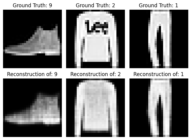
model.eval()  # put in evaluation mode - no gradients
examples = enumerate(fmnist_test_loader)
batch_idx, (example_data, example_targets) = next(examples)
print("shape: \n", example_data.shape)
fig = plt.figure()
for i in range(3):
    ax = fig.add_subplot(2,3,i+1)
    ax.imshow(example_data[i][0], cmap='gray', interpolation='none')
    ax.set_title("Ground Truth: {}".format(example_targets[i]))
    ax.set_axis_off()

    ax = fig.add_subplot(2,3,i+4)
    recon_img = model(example_data[i][0].view(1, -1).to(device)).data.cpu().numpy().reshape(28, 28)
    ax.imshow(recon_img, cmap='gray')
    ax.set_title("Reconstruction of: {}".format(example_targets[i]))
    ax.set_axis_off()
plt.tight_layout()

shape: 
 torch.Size([64, 1, 28, 28])

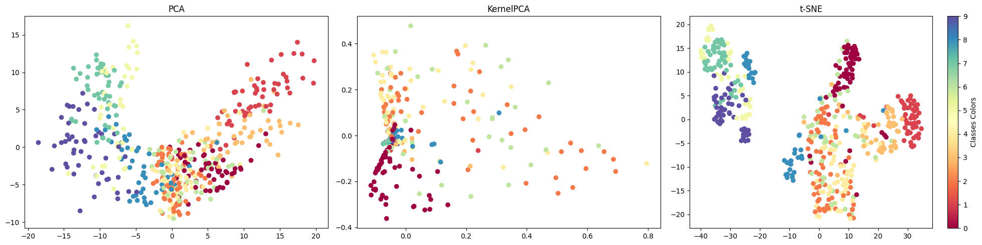
# let's compare different dimensionality reduction methods
n_neighbors = 10
n_components = 2
n_points = 500

fmnist_test_loader = torch.utils.data.DataLoader(dataset=fmnist_test_dataset,
                                          batch_size=n_points, 
                                          shuffle=False)
X, labels = next(iter(fmnist_test_loader))
latent_X = model.get_latent_rep(X.to(device).view(n_points, -1)).data.cpu().numpy()
labels = labels.data.cpu().numpy()

# scikit-learn imports
from sklearn.manifold import LocallyLinearEmbedding, Isomap, TSNE
from sklearn.decomposition import PCA, KernelPCA
import numpy as np

fig = plt.figure(figsize=(20,5))

# PCA
t0 = time.time()
x_pca = PCA(n_components).fit_transform(latent_X)
t1 = time.time()
print("PCA time: %.2g sec" % (t1 - t0))
ax = fig.add_subplot(1, 3, 1)
ax.scatter(x_pca[:, 0], x_pca[:, 1], c=labels, cmap=plt.cm.Spectral)
ax.set_title('PCA')

# KPCA
t0 = time.time()
x_kpca = KernelPCA(n_components, kernel='rbf').fit_transform(latent_X)
t1 = time.time()
print("KPCA time: %.2g sec" % (t1 - t0))
ax = fig.add_subplot(1, 3, 2)
ax.scatter(x_kpca[:, 0], x_kpca[:, 1], c=labels, cmap=plt.cm.Spectral)
ax.set_title('KernelPCA')

# t-SNE
t0 = time.time()
x_tsne = TSNE(n_components).fit_transform(latent_X)
t1 = time.time()
print("t-SNE time: %.2g sec" % (t1 - t0))
ax = fig.add_subplot(1, 3, 3)
scatter = ax.scatter(x_tsne[:, 0], x_tsne[:, 1], c=labels, cmap=plt.cm.Spectral)
ax.set_title('t-SNE')

bounds = np.linspace(0, 10, 11)
cb = plt.colorbar(scatter, spacing='proportional',ticks=bounds)
cb.set_label('Class Colors')

plt.tight_layout()

PCA time: 0.0079 sec
KPCA time: 0.023 sec
t-SNE time: 0.39 sec

Credits

• Icons made by Becris from www.flaticon.com
• Icons from Icons8.com – https://icons8.com
• Datasets from Kaggle – https://www.kaggle.com/
• Jason Brownlee – Why Initialize a Neural Network with Random Weights?
• OpenAI – Deep Double Descent
• Tal Daniel