
Learning Methods of Deep Learning
Created by Deepfinder
 Agenda
- Learning from a Teacher: Supervised Learning
- Inferring the Whole from the Small: Unsupervised Learning
- Learning Without a Teacher: Self-supervised Learning
- Expanding from a Few Labels: Semi-supervised Learning
- Distinguishing Similarities and Differences: Contrastive Learning
- Applying Knowledge by Analogy: Transfer Learning
- Confronting an Opponent: Adversarial Learning
- Strength in Numbers: Ensemble Learning
- Different Paths, One Goal: Federated Learning
- Persevering Through Trial and Error: Reinforcement Learning
- Eager to Learn: Active Learning
- Learning to Learn: Meta-Learning
Tutorial 01 – Learning from a Teacher: Supervised Learning
 The Perceptron
-
One of the first and simplest linear models.
-
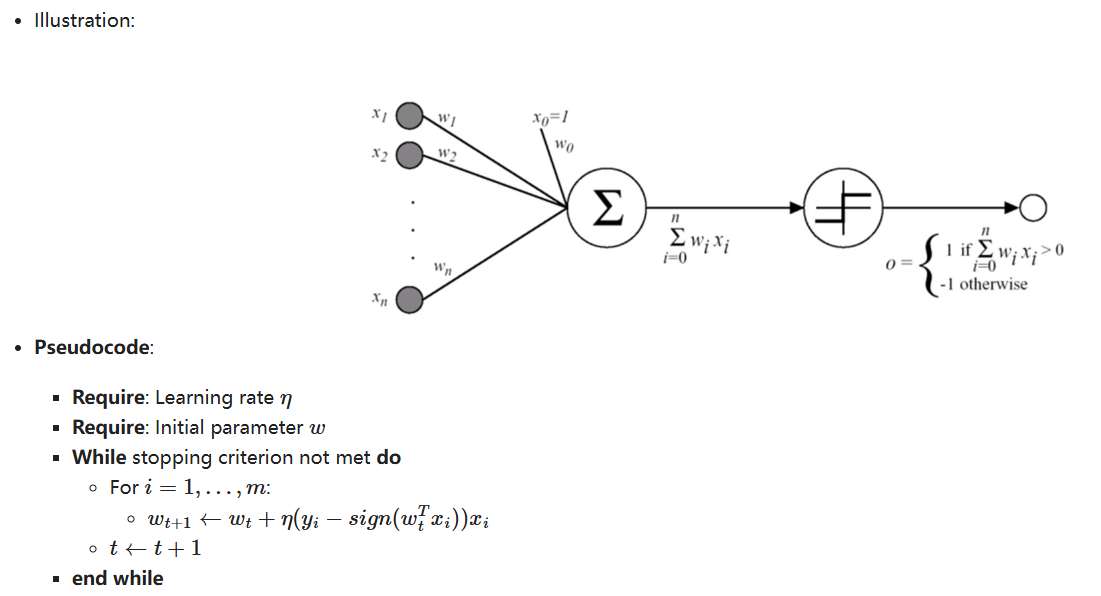
Based on a linear threshold unit (LTU): the inputs and outputs are numbers, and each connection is associated with a weight.
-
The LTU computes a weighted sum of its inputs: $z = w_1x_1 + w_2x_2 +….+w_nx_n = w^Tx$, then applies a step function to that sum and outputs the result: $$ h_w(x) = step(z) = step(w^Tx) $$
-
Illustration:
-
Pseudocode:
- Require: Learning rate $eta$
- Require: Initial parameter $w$
- While stopping criterion not met do
- For $i=1,…,m$:
- $ w_{t+1} leftarrow w_t +eta(y_i -sign(w_t^Tx_i))x_i $
- $t leftarrow t + 1$
- For $i=1,…,m$:
- end while
 Multi-Layer Perceptron (MLP)
-
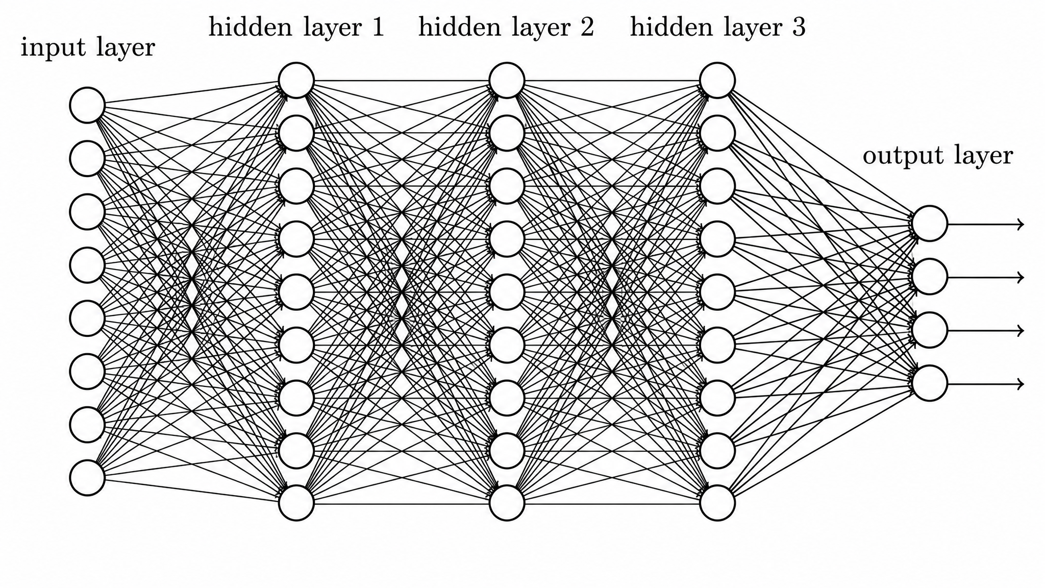
An MLP consists of an input layer, one or more hidden layers, and a final output layer.
-
When the number of hidden layers is greater than 2, the network is usually called a deep neural network (DNN); with fewer than 2 hidden layers, it is commonly referred to as an MLP. This is a general convention rather than a strict definition.
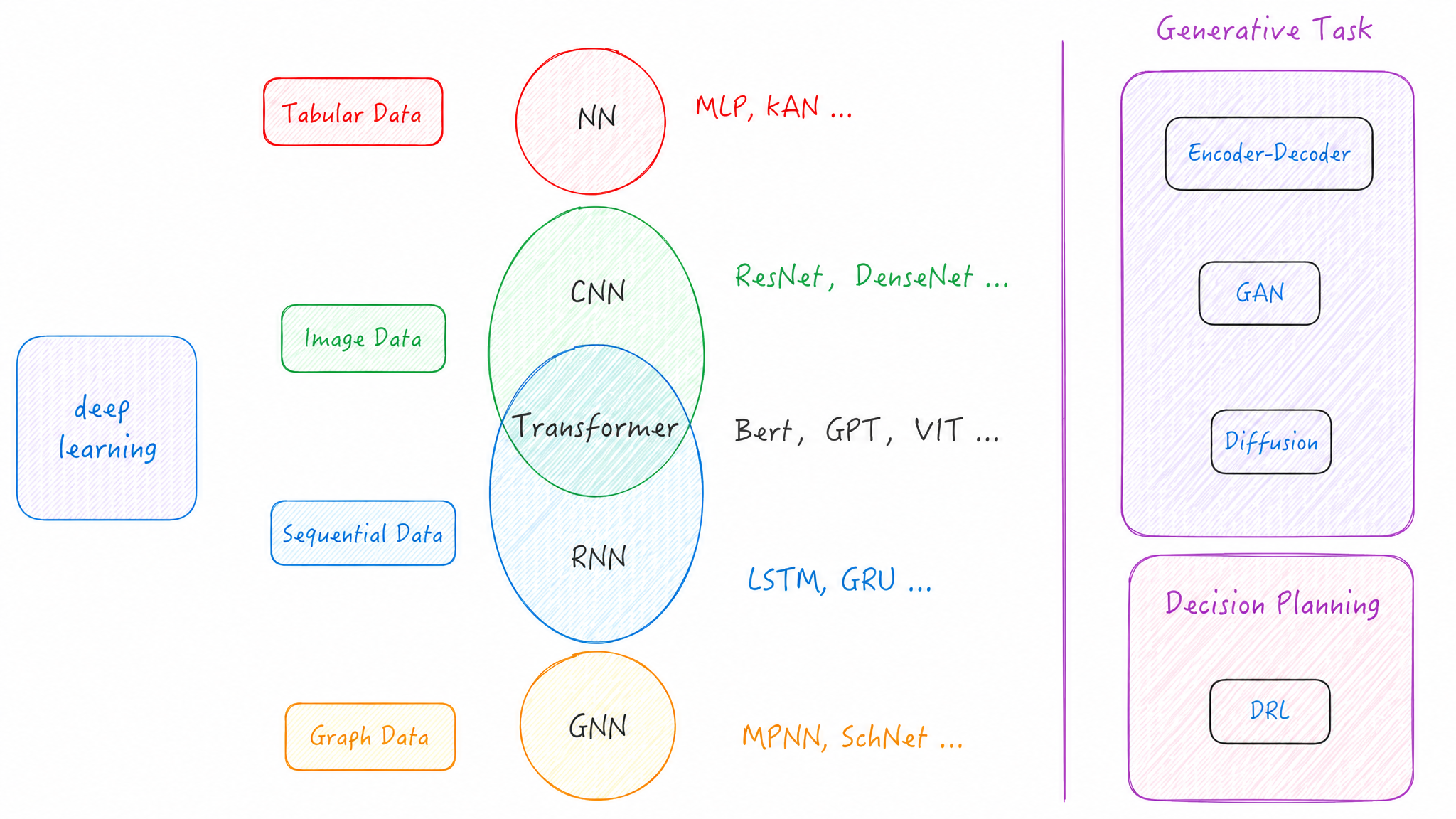
Various deep learning algorithms and models can be derived from the MLP.
 Training Logic of Deep Learning Algorithms and Models
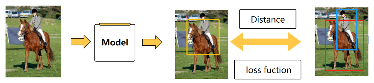
 Forward calculation
-
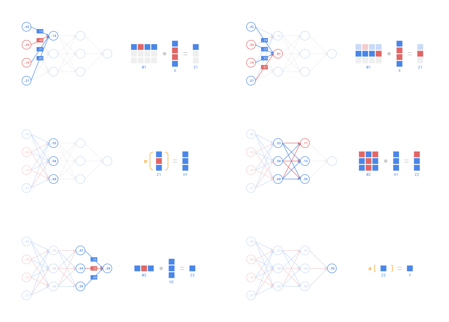
During the forward pass, for each training instance, the algorithm feeds it into the network and computes the output of every neuron in each successive layer.
-
Using the network to make predictions is simply performing a forward pass.
An example is shown below:
 Backpropagation
Backpropagation is an efficient method for computing gradients. It can quickly calculate the partial derivative for each neuron in a network. The algorithm first computes the network output through forward propagation, then propagates the error backward from the output layer to the input layer, and finally calculates each neuron’s partial derivative based on that error. The core idea of backpropagation is to use the chain rule to pass the error backward and compute each neuron’s contribution to it.
An example is shown below:
Initialize the network by constructing a neural network with only one layer.

(1) Initialize the network parameters:
Assume that the initialized input and output values of the neural network are: $x_1=0.5, x_2=1.0, y=0.8$.
The initialized parameters are: $w_1=1.0, w_2=0.5, w_3=0.5, w_4=0.7, w_5=1.0, w_6=2.0$.
(2) Perform the forward calculation, as shown below.
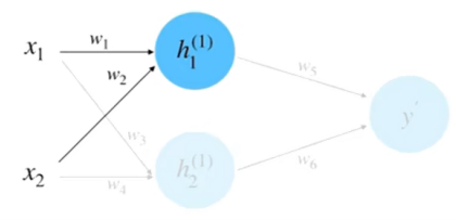
Similarly, $h_2$ is calculated as 0.95. Multiply $h_1$ and $h_2$ by the corresponding weights and sum them to obtain the forward propagation result, as shown below.
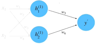
$$
begin{aligned}
y^{prime} & =w_5 cdot h_1^{(1)}+w_6 cdot h_2^{(1)}
& =1.0 cdot 1.0+2.0 cdot 0.95
& =2.9
end{aligned}
$$
(3) Calculate the loss: based on the true data value $y=0.8$ and the squared error loss function, the loss is computed as follows.
$$
begin{aligned}
delta & =frac{1}{2}left(y-y^{prime}right)^2
& =0.5(0.8-2.9)^2
& =2.205
end{aligned}
$$
(4) Calculate the gradient: this process is essentially the calculation of partial derivatives. Taking the partial derivative with respect to parameter $w_5$ as an example, the process is shown below.
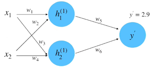
According to the chain rule:
$$
frac{partial delta}{partial w_5}=frac{partial delta}{partial y^{prime}} cdot frac{partial y^{prime}}{partial w_5}
$$
Where:
$$
begin{aligned}
frac{partial delta}{partial y^{prime}} & =2 cdot frac{1}{2} cdotleft(y-y^{prime}right)(-1)
& =y^{prime}-y
& =2.9-0.8
& =2.1
y^{prime} & =w_5 cdot h_1^{(1)}+w_6 cdot h_2^{(1)}
frac{partial y^{prime}}{partial w_5} & =h_1^{(1)}+0
& =1.0
end{aligned}
$$
Therefore:
$$
frac{partial delta}{partial w_5}=frac{partial delta}{partial y^{prime}} cdot frac{partial y^{prime}}{partial w_5}=2.1 times 1.0=2.1
$$
Similarly, if we take parameter $w_1$ as an example, its partial derivative calculation also uses the chain rule, as shown below.
$$
begin{gathered}
frac{partial delta}{partial w_1}=frac{partial delta}{partial y^{prime}} cdot frac{partial y^{prime}}{partial h_1^{(1)}} cdot frac{partial h_1^{(1)}}{partial w_1}
y^{prime}=w_5 cdot h_1^{(1)}+w_6 cdot h_2^{(1)}
frac{partial y^{prime}}{partial h_1^{(1)}}=w_5+0
=1.0
h_1^{(1)}=w_1 cdot x_1+w_2 cdot x_2
frac{partial h_1^{(1)}}{partial w_1}=x_1+0
frac{partial delta}{partial w_1}=frac{partial delta}{partial y^{prime}} cdot frac{partial y^{prime}}{partial h_1^{(1)}} cdot frac{partial h_1^{(1)}}{partial w_1}=2.1 times 1.0 times 0.5=1.05
end{gathered}
$$
(5) Update the network parameters with gradient descent: suppose the initial value of the hyperparameter “learning rate” is 0.1. According to the gradient descent update formula, the update for parameter $w_1$ is calculated as follows:
$$
w_1^{text {(update) }}=w_1-eta cdot frac{partial delta}{partial w_1}=1.0-0.1 times 1.05=0.895
$$
Similarly, the other updated parameters can be calculated as:
$$
w_1=0.895, w_2=0.895, w_3=0.29, w_4=0.28, w_5=0.79, w_6=1.8005
$$
At this point, we have completed the full parameter-iteration process. We can calculate the loss to see whether it has decreased, as follows:
$$
begin{aligned}
delta & =frac{1}{2}left(y-y^{prime}right)^2
& =0.5(0.8-1.3478)^2
& =0.15
end{aligned}
$$
Compared with the previous forward propagation loss of 2.205, this result is clearly much smaller.
import torch
import torch.nn as nn
import torch.optim as optim
import torchvision
import torchvision.transforms as transforms

# 1. Hyperparameter settings
batch_size = 64
learning_rate = 0.001
num_epochs = 2  # For this example, the number of epochs is kept small; increase it if needed

# 2. Data loading and preprocessing
# MNIST contains 28x28 grayscale images; here we apply simple transforms such as tensor conversion and normalization
transform = transforms.Compose([
    transforms.ToTensor(),  # Convert a PIL Image or numpy.ndarray into a tensor
    transforms.Normalize((0.1307,), (0.3081,))  # Normalize using the official MNIST mean and standard deviation
])

train_dataset = torchvision.datasets.MNIST(
    root='./data',
    train=True,
    transform=transform,
    download=True
)
test_dataset = torchvision.datasets.MNIST(
    root='./data',
    train=False,
    transform=transform,
    download=True
)

train_loader = torch.utils.data.DataLoader(
    dataset=train_dataset,
    batch_size=batch_size,
    shuffle=True
)
test_loader = torch.utils.data.DataLoader(
    dataset=test_dataset,
    batch_size=batch_size,
    shuffle=False
)

# 3. Define the network architecture
class SimpleNN(nn.Module):
    def __init__(self):
        super(SimpleNN, self).__init__()
        # MNIST input images have shape 1x28x28; first flatten them to (batch_size, 784)
        self.flatten = nn.Flatten()

        self.fc1 = nn.Linear(28 * 28, 128)
        self.relu1 = nn.ReLU()

        self.fc2 = nn.Linear(128, 64)
        self.relu2 = nn.ReLU()

        self.fc3 = nn.Linear(64, 10)  # 10 classes (digits 0-9)

    def forward(self, x):
        x = self.flatten(x)
        x = self.fc1(x)
        x = self.relu1(x)
        x = self.fc2(x)
        x = self.relu2(x)
        x = self.fc3(x)
        return x

# 4. Initialize the model, loss function, and optimizer
device = torch.device("cuda" if torch.cuda.is_available() else "cpu")
model = SimpleNN().to(device)
criterion = nn.CrossEntropyLoss()  # Cross-entropy loss is commonly used for classification tasks
optimizer = optim.Adam(model.parameters(), lr=learning_rate)

# 5. Training function
def train_one_epoch(model, dataloader, criterion, optimizer, device):
    model.train()  # Set the model to training mode
    running_loss = 0.0
    correct = 0
    total = 0

    for images, labels in dataloader:
        images, labels = images.to(device), labels.to(device)

        # Forward pass
        outputs = model(images)
        loss = criterion(outputs, labels)

        # Backpropagation and optimization
        optimizer.zero_grad()
        loss.backward()
        optimizer.step()

        # Track loss and accuracy
        running_loss += loss.item() * images.size(0)
        _, predicted = torch.max(outputs, 1)
        correct += (predicted == labels).sum().item()
        total += labels.size(0)

    epoch_loss = running_loss / total
    epoch_acc = correct / total
    return epoch_loss, epoch_acc

# 6. Test function
def evaluate(model, dataloader, criterion, device):
    model.eval()  # Set the model to evaluation mode
    running_loss = 0.0
    correct = 0
    total = 0

    # No gradients are needed during evaluation
    with torch.no_grad():
        for images, labels in dataloader:
            images, labels = images.to(device), labels.to(device)

            outputs = model(images)
            loss = criterion(outputs, labels)

            running_loss += loss.item() * images.size(0)
            _, predicted = torch.max(outputs, 1)
            correct += (predicted == labels).sum().item()
            total += labels.size(0)

    epoch_loss = running_loss / total
    epoch_acc = correct / total
    return epoch_loss, epoch_acc

# 7. Training and validation
for epoch in range(num_epochs):
    train_loss, train_acc = train_one_epoch(model, train_loader, criterion, optimizer, device)
    test_loss, test_acc = evaluate(model, test_loader, criterion, device)

    print(f"Epoch [{epoch+1}/{num_epochs}] "
          f"Train Loss: {train_loss:.4f}, Train Acc: {train_acc:.4f}, "
          f"Test Loss: {test_loss:.4f}, Test Acc: {test_acc:.4f}")
/home/arwin/anaconda3/envs/dl/lib/python3.8/site-packages/tqdm/auto.py:21: TqdmWarning: IProgress not found. Please update jupyter and ipywidgets. See https://ipywidgets.readthedocs.io/en/stable/user_install.html
from .autonotebook import tqdm as notebook_tqdm
Epoch [1/2] Train Loss: 0.2726, Train Acc: 0.9208, Test Loss: 0.1360, Test Acc: 0.9585
Epoch [2/2] Train Loss: 0.1135, Train Acc: 0.9654, Test Loss: 0.0978, Test Acc: 0.9690 Credits
- Icons made by Becris from www.flaticon.com
- Icons from Icons8.com – https://icons8.com
- Datasets from Kaggle – https://www.kaggle.com/
- Jason Brownlee – Why Initialize a Neural Network with Random Weights?
- OpenAI – Deep Double Descent
- Tal Daniel