
Learning Methods of Deep Learning
created by Deepfinder
 Agenda
- Learning from a Teacher: Supervised Learning
- Seeing the Pattern: Unsupervised Learning
- Learning Without Labels: Self-supervised Learning
- Learning from a Few Labels: Semi-supervised Learning
- Learning by Comparison: Contrastive Learning
- Learning by Transfer: Transfer Learning
- Learning Through Competition: Adversarial Learning
- Working Together: Ensemble Learning
- Different Paths, One Goal: Federated Learning
- Learning Through Trial and Error: Reinforcement Learning
- Eager to Learn: Active Learning
- Learning to Learn: Meta-Learning
 The Adversarial Mechanism
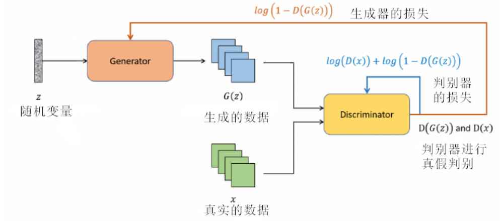
Generative adversarial networks (GANs) are a revolutionary idea in deep learning. They provide a new way to generate data. The word adversarial describes the core idea: two neural networks compete with each other to generate data.
These two networks are the Generator and the Discriminator.
Imagine a GAN as a carefully arranged art performance. On the stage, there are two main artists: the generator and the discriminator.
-
The generator is full of creativity. It creates something from nothing. It starts from a random inspiration, or noise vector, and tries to make convincing works.
-
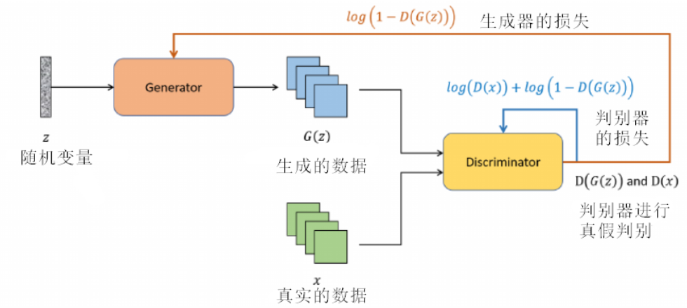
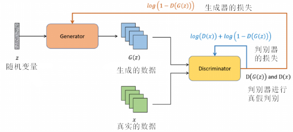
On the other side of the stage, the discriminator acts as a critic. It has sharp eyes and does not miss small flaws. When it sees a work from the real world, it accepts it. When it sees a work from the generator, it checks it carefully and decides whether it is real or fake. This judgment is sent back to the generator. It tells the generator what is not good enough and what needs to be improved.
-
This dance is an iterative process. Both sides challenge each other and improve together.
-
Over time, the generator becomes more skilled. The discriminator also becomes better at judging. In the end, we hope the generator can create works of such high quality that even the sharpest critic, the discriminator, cannot tell whether they are real or fake.
More specifically:
In a GAN, the generator plays the role of a creative artist. This “artist” draws inspiration from a random vector. It passes the vector through several neural network layers, such as convolutional layers or fully connected layers, and turns it into a visible output. A real artist improves by practicing and correcting mistakes. In the same way, the generator keeps adjusting its parameters so that its outputs become more realistic. Its goal is to create convincing data, so that the discriminator, a strict art critic, finds it hard to tell whether the data is real or fake. Therefore, the generator is not only a creator. It is also a lifelong learner that keeps improving its “art skills” through feedback from the discriminator.
The discriminator is the strict art critic. It checks every work carefully. Inside it, several neural network layers, such as convolutional layers or fully connected layers, form a complex decision system. This system decides whether a work is a real sample from the real world or an imitation made by the generator. After receiving data, the discriminator outputs a score through its network. This score represents the probability that the data is real. Its main task is to correctly identify real data and generated data. Its judgment also gives valuable feedback to the generator, so the generator can further improve its creation skills. Therefore, the discriminator is both a strict judge and an important guide for the generator.
import torch as t
from torch import nn
from torch.autograd import Variable
from torch.optim import Adam
from torchvision import transforms
from torchvision.utils import make_grid
from torchvision.datasets import CIFAR10, MNIST
from pylab import plt
%matplotlib inline
class Config:
lr = 0.0002
nz = 100 # noise dimension
image_size = 64
image_size2 = 64
nc = 1 # chanel of img
ngf = 64 # generate channel
ndf = 64 # discriminative channel
beta1 = 0.5
batch_size = 32
max_epoch = 10 # =1 when debug
workers = 2
gpu = True # use gpu or not
opt=Config()
# data preprocess
transform=transforms.Compose([
transforms.Resize(opt.image_size),
transforms.ToTensor(),
transforms.Normalize([0.5], [0.5])
])
dataset=MNIST(root='data', transform=transform, download=True)
# dataloader with multiprocessing
dataloader=t.utils.data.DataLoader(dataset,
opt.batch_size,
shuffle=True,
num_workers=opt.workers)
# define model
netg = nn.Sequential(
nn.ConvTranspose2d(opt.nz,opt.ngf*8,4,1,0,bias=False),
nn.BatchNorm2d(opt.ngf*8),
nn.ReLU(True),
nn.ConvTranspose2d(opt.ngf*8,opt.ngf*4,4,2,1,bias=False),
nn.BatchNorm2d(opt.ngf*4),
nn.ReLU(True),
nn.ConvTranspose2d(opt.ngf*4,opt.ngf*2,4,2,1,bias=False),
nn.BatchNorm2d(opt.ngf*2),
nn.ReLU(True),
nn.ConvTranspose2d(opt.ngf*2,opt.ngf,4,2,1,bias=False),
nn.BatchNorm2d(opt.ngf),
nn.ReLU(True),
nn.ConvTranspose2d(opt.ngf,opt.nc,4,2,1,bias=False),
nn.Tanh()
)
netd = nn.Sequential(
nn.Conv2d(opt.nc,opt.ndf,4,2,1,bias=False),
nn.LeakyReLU(0.2,inplace=True),
nn.Conv2d(opt.ndf,opt.ndf*2,4,2,1,bias=False),
nn.BatchNorm2d(opt.ndf*2),
nn.LeakyReLU(0.2,inplace=True),
nn.Conv2d(opt.ndf*2,opt.ndf*4,4,2,1,bias=False),
nn.BatchNorm2d(opt.ndf*4),
nn.LeakyReLU(0.2,inplace=True),
nn.Conv2d(opt.ndf*4,opt.ndf*8,4,2,1,bias=False),
nn.BatchNorm2d(opt.ndf*8),
nn.LeakyReLU(0.2,inplace=True),
nn.Conv2d(opt.ndf*8,1,4,1,0,bias=False),
nn.Sigmoid()
) GAN Model and Loss Explained
For a traditional GAN, the objective function is a two-player zero-sum game. The generator ( $G$ ) and the discriminator ( $D$ ) have opposite goals. The game can be written as:
$$
min _G max _D mathcal{L}(D, G)=mathrm{E}_{x sim p_{text {data }}(x)}[log D(x)]+mathrm{E}_{z sim p_z(z)}[log (1-D(G(z)))]
$$
- The outer minimization (min) represents the goal of the generator $G$. The generator wants to minimize the probability that the discriminator correctly classifies its generated samples. In other words, the generator tries to fool the discriminator and make it believe that generated samples are real.
- The inner maximization (max) represents the goal of the discriminator $D$. The discriminator wants to maximize its ability to classify real and generated samples.
The core idea of a GAN is to build a competition between the generator and the discriminator. To make this competition work, we need to define suitable loss functions for both networks. In the most basic GAN, the generator produces data that can fool the discriminator. More specifically, the generator wants the discriminator to think that generated data is as close to real data as possible. Therefore, the generator loss is usually based on the discriminator’s evaluation of generated data.
Assume that $G$ is the generator and $D$ is the discriminator. Given a random noise vector $z$, the generator $G$ produces data $G(z)$.
The discriminator $D$ evaluates this data and outputs a probability $D(G(z))$. This value means how likely it thinks $G(z)$ is real data.
The generator wants $D(G(z))$ to be as close to 1 as possible. This means the discriminator is fooled and believes that the generated data is real.
Considering the generator alone:
If we only consider images produced by the generator and ignore the influence of real data $left(mathrm{E}_{x sim p_{d: 18}(x)}[log D(x)]=0right)$, the original GAN loss can be simplified as:
$$
L_G=mathrm{E}_{z sim p_z(z)}[log (1-D(G(z)))]
$$
Formula explanation:
- When $D(G(z))$ is close to 1, the discriminator is almost fully sure that the generated data is real. Then $1-D(G(z))$ is close to 0, and $log (1-D(G(z)))$ becomes a large negative value. This is exactly what we want when minimizing the generator loss.
- When $D(G(z))$ is close to 0, the discriminator thinks the generated data is fake. In this case, $1-D(G(z))$ is close to 1, so $log (1-D(G(z)))$ is close to 0. The generator tries to avoid this situation. Its goal is to minimize $log (1-D(G(z)))$, which encourages it to produce data that can fool the discriminator.
 Why is there a log in the loss formula?
Considering the discriminator alone:
If we only look from the discriminator’s perspective, the GAN loss mainly focuses on how the discriminator separates real data from generated data. For the discriminator $D$, the loss function is:
$$
L_D=mathrm{E}_{x sim p_{text {data }}(x)}[log D(x)]+mathrm{E}_{z sim p_z(z)}[log (1-D(G(z)))]
$$
The loss function has two parts:
(1) $mathrm{E}_{x sim p_{text {data}}(x)}[log D(x)]$: this part is about real data. The discriminator $D$ tries to maximize the probability of correctly classifying real data samples $x$. In other words, for samples $x$ from the real data distribution, it wants to output values as close to 1 as possible.
(2) $mathrm{E}_{z sim p_(z)}[log (1-D(G(z)))]$: this part is about generated data. The discriminator $D$ tries to maximize the probability of correctly classifying generated data as fake. This means that for fake samples generated by $G$ from noise sampled from the prior noise distribution $p_z$, the discriminator output should be as close to 0 as possible.
The goal of the discriminator $D$ is to maximize the loss function. This means that, for the best result, the discriminator wants to accurately distinguish real data from generated data. In the ideal case, for real data, $D(x)=1$; for generated data, $D(G(x))=0$.
In real training, however, this ideal case is rarely reached. The generator is also improving itself and producing more realistic samples to fool the discriminator.
# optimizer
optimizerD = Adam(netd.parameters(),lr=opt.lr,betas=(opt.beta1,0.999))
optimizerG = Adam(netg.parameters(),lr=opt.lr,betas=(opt.beta1,0.999))

# criterion
criterion = nn.BCELoss()

fix_noise = Variable(t.FloatTensor(opt.batch_size,opt.nz,1,1).normal_(0,1))
if opt.gpu:
    fix_noise = fix_noise.cuda()
    netd.cuda()
    netg.cuda()
    criterion.cuda()
Training a GAN Model
Before training a GAN model, we first need to choose a suitable neural network structure. For example, for image generation, convolution-based structures are common. The weights of the generator $G$ and discriminator $D$ are usually initialized with small random values. A GAN contains two networks: the generator and the discriminator. They need to be trained alternately or at the same time. The training loop of a GAN is roughly as follows:
- First, train the discriminator. Use real data and fake data generated by the current generator to train the discriminator. The discriminator’s goal is to correctly distinguish real data from fake data.
More specifically, on one side, sample a batch of data $x$ from the real data distribution. Compute the discriminator output $D(x)$ on real data, and compute the loss $mathrm{E}_{x sim p_{text {deta }}(x)}[log D(x)]$. On the other side, sample a batch of noise $z$ from the random noise distribution. Use the generator $G$ to produce a batch of fake data $G(z)$. Compute the discriminator output $D(G(z))$ on the fake data, and compute the loss $mathrm{E}_{z sim p_z(z)}[log (1-D(G(z)))]$. Combine the losses from real data and generated data, and use the total loss to update the weights of the discriminator $D$. Optimizers such as Adam or RMSProp are often used.
- Then train the generator. It tries to fool the discriminator and make it believe that generated data is real. The generator’s goal is to generate data that the discriminator misclassifies as real data.
More specifically, sample another batch of noise $Z$ from the random noise distribution. Use the discriminator $D$ to evaluate the fake data produced by the generator $G$. Compute the loss $mathrm{E}_{z sim p_z(z)}[log (1-D(G(z)))]$, and use this loss to update the weights of the generator $G$.
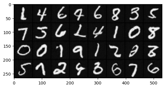
Every few epochs, we can use some metrics to evaluate the output of the generator. Repeat the training steps above until a stopping condition is met. This can be a fixed number of training epochs, a model performance threshold, or another condition. If the condition is not met, return to the start of the training loop.
During this loop, both the generator and the discriminator gradually improve and try to perform their tasks better. The final goal is to find a balance point where generated data is almost impossible to distinguish from real data. This gradual and repeated training method lets the model learn from data and adapt to it. This is a key reason why many machine learning algorithms work well.
import matplotlib.pyplot as plt

# Store the loss for each iteration
losses_D = []
losses_G = []

for epoch in range(opt.max_epoch):
    for ii, data in enumerate(dataloader, 0):
        real, _ = data
        input = Variable(real)  # Wrap real images as PyTorch variables for the computation graph
        label = Variable(t.ones(input.size(0)))  # Create label variables with the same count as real images. All values are 1, meaning real data
        noise = t.randn(input.size(0), opt.nz, 1, 1)  # Generate random noise with the same count as real images, used to create fake images
        noise = Variable(noise)  # Wrap random noise as a PyTorch variable for the computation graph

        if opt.gpu:
            noise = noise.cuda()
            input = input.cuda()
            label = label.cuda()

        # ----- train netd -----
        netd.zero_grad()
        ## train netd with real img
        output = netd(input)
        error_real = criterion(output.squeeze(), label)
        error_real.backward()
        D_x = output.data.mean()
        ## train netd with fake img
        fake_pic = netg(noise).detach()
        output2 = netd(fake_pic)
        label.data.fill_(0)  # 0 for fake
        error_fake = criterion(output2.squeeze(), label)
        error_fake.backward()
        D_x2 = output2.data.mean()
        error_D = error_real + error_fake
        optimizerD.step()

        # ------ train netg -------
        netg.zero_grad()
        label.data.fill_(1)
        noise.data.normal_(0, 1)
        fake_pic = netg(noise)
        output = netd(fake_pic)
        error_G = criterion(output.squeeze(), label)
        error_G.backward()
        optimizerG.step()
        D_G_z2 = output.data.mean()

        # Store loss values
        losses_D.append(error_D.item())
        losses_G.append(error_G.item())

        if ii % 500 == 0:
            print(f"Iteration {ii}/{epoch}: "
                  f"Discriminator Loss: {error_D.item():.4f}, "
                  f"Generator Loss: {error_G.item():.4f}, "
                  f"D(x): {D_x:.4f}, "
                  f"D(G(z)) (on fake data): {D_G_z2:.4f}, "
                  f"D(G(z)) (on real data): {D_x2:.4f}")
    if epoch % 2 == 0:
        fake_u = netg(fix_noise)
        imgs = make_grid(fake_u.data * 0.5 + 0.5).cpu()  # CHW
        plt.imshow(imgs.permute(1, 2, 0).numpy())  # HWC
        plt.show()

# Plot the loss curves
plt.figure(figsize=(10, 5))
plt.title("Generator and Discriminator Loss During Training")
plt.plot(losses_G, label="G")
plt.plot(losses_D, label="D")
plt.xlabel("iterations")
plt.ylabel("Loss")
plt.legend()
plt.show()
Iteration 0/0: Discriminator Loss: 0.0084, Generator Loss: 6.3695, D(x): 0.9990, D(G(z)) (on fake data): 0.0050, D(G(z)) (on real data): 0.0072
Iteration 500/0: Discriminator Loss: 0.0135, Generator Loss: 5.0962, D(x): 0.9909, D(G(z)) (on fake data): 0.0149, D(G(z)) (on real data): 0.0044
Iteration 1000/0: Discriminator Loss: 0.0010, Generator Loss: 7.0314, D(x): 0.9996, D(G(z)) (on fake data): 0.0019, D(G(z)) (on real data): 0.0006
Iteration 1500/0: Discriminator Loss: 0.7012, Generator Loss: 1.0979, D(x): 0.6444, D(G(z)) (on fake data): 0.4389, D(G(z)) (on real data): 0.1342
Iteration 0/1: Discriminator Loss: 0.0329, Generator Loss: 3.9298, D(x): 0.9901, D(G(z)) (on fake data): 0.0524, D(G(z)) (on real data): 0.0220
Iteration 500/1: Discriminator Loss: 0.0065, Generator Loss: 6.4350, D(x): 0.9996, D(G(z)) (on fake data): 0.0025, D(G(z)) (on real data): 0.0060
Iteration 1000/1: Discriminator Loss: 0.2043, Generator Loss: 4.6965, D(x): 0.9954, D(G(z)) (on fake data): 0.0191, D(G(z)) (on real data): 0.1569
Iteration 1500/1: Discriminator Loss: 0.0110, Generator Loss: 6.9614, D(x): 0.9992, D(G(z)) (on fake data): 0.0025, D(G(z)) (on real data): 0.0101
Iteration 0/2: Discriminator Loss: 0.0039, Generator Loss: 8.1376, D(x): 0.9999, D(G(z)) (on fake data): 0.0004, D(G(z)) (on real data): 0.0039
Iteration 500/2: Discriminator Loss: 0.0001, Generator Loss: 9.3291, D(x): 1.0000, D(G(z)) (on fake data): 0.0001, D(G(z)) (on real data): 0.0001
Iteration 1000/2: Discriminator Loss: 0.0001, Generator Loss: 9.8352, D(x): 1.0000, D(G(z)) (on fake data): 0.0001, D(G(z)) (on real data): 0.0001
Iteration 1500/2: Discriminator Loss: 0.0001, Generator Loss: 9.6669, D(x): 1.0000, D(G(z)) (on fake data): 0.0001, D(G(z)) (on real data): 0.0001 Improved GAN
“Improved Techniques for Training GANs” is a paper published by Ian J. Goodfellow and his colleagues in 2016. The paper proposed important improvements to the training process of generative adversarial networks (GANs). These improvements mainly focus on making GAN training more stable and improving performance. They also address common problems in early GAN training, such as mode collapse.
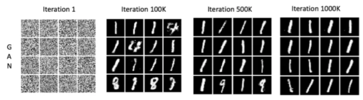
When training a GAN, we ideally want the generator to learn many aspects of the data distribution. Then it can produce diverse and realistic data. Mode collapse means that the generator starts to produce only a very limited set of samples. These samples may still fool the discriminator with a high success rate. In other words, the generator finds a “shortcut”. It only generates certain specific samples, which may be hard for the current discriminator to recognize as fake, and ignores other features and diversity in the data. As a result, the generated data may look realistic, but it lacks diversity.
The main reason for mode collapse is the instability of GAN models. For example, if the discriminator learns too quickly, the generator may find and repeatedly use a few specific patterns that can pass the discriminator, instead of learning a more diverse data generation strategy. In short, if the training between the generator and the discriminator is not balanced, one side may become too strong. This can push the other side to use extreme strategies.
The root of this instability is that GAN training is essentially a game between two networks, the generator and the discriminator. This process can be very unstable. In theory, the two sides should reach a Nash equilibrium. In practice, this is often hard to achieve. For example:
- If the discriminator is too strong, it can easily identify the generator’s outputs, no matter how good they are. This gives the generator gradient signals that are too strong and too sharp. The generator may not find a useful direction to improve generation quality. It can get stuck and fail to produce realistic enough data.
- If the discriminator is too weak, it cannot provide accurate enough feedback to the generator. Then the generator may still “pass” even when it produces low-quality outputs. It will not have enough motivation to improve and learn to generate higher-quality data.
Imagine a student learning to draw very realistic landscape paintings to “fool” a teacher. The teacher’s task is to decide whether each painting was drawn by the student or by a real artist. If the teacher is very experienced, meaning the discriminator is too strong, it can easily recognize all of the student’s paintings, no matter their quality. This creates several problems:
- The student, or generator, may feel discouraged. The student may lose motivation or direction because their work is always recognized as fake. They may not know how to improve. Also, there is no useful feedback. The teacher may only say “this is wrong” without giving specific suggestions. This makes it hard for the student to learn how to improve their drawing skills.
- If the teacher has weak judgment, meaning the discriminator is too weak, the student lacks challenge. If the teacher almost always thinks the student’s work was made by a real artist, the student may believe they have already “mastered” the skill, even though the work quality is not high. Without enough challenge and accurate feedback, the student may stop improving or may not know which parts need more work.
Solutions to mode collapse:
Feature matching
Minibatch discrimination
One-sided label smoothing
Virtual batch normalization Credits
- Icons made by Becris from www.flaticon.com
- Icons from Icons8.com – https://icons8.com
- Dive Into Deep Learning – Recurrent Neural Networks
- DS-GA 1008 – NYU CENTER FOR DATA SCIENCE – Deep Sequence Modeling
- Text classification with the torchtext library
- Tricks For Training Transformers – Borealis AI – P. Xu, S. Prince
- Tal Daniel