
Learning Methods of Deep Learning
created by Deepfinder
 Agenda
- Learning from a Teacher: Supervised Learning
- Seeing the Pattern: Unsupervised Learning
- Learning Without a Teacher: Self-supervised Learning
- Learning from a Few Labels: Semi-supervised Learning
- Distinguishing Similarities and Differences: Contrastive Learning
- Learning by Transfer: Transfer Learning
- Confronting the Opponent: Adversarial Learning
- Strength in Numbers: Ensemble Learning
- Different Paths, Same Goal: Federated Learning
- Learning Through Persistence: Reinforcement Learning
- Eager to Learn: Active Learning
- Learning How to Learn: Meta-Learning
Tutorial 06 – Learning by Transfer: Transfer Learning
 Applications of Transfer Learning
Domain Adaptation – adapting across domains:
-
Core idea: transfer or adapt knowledge learned in one domain, called the source domain, to another different but related domain, called the target domain.
-
Computer vision example: in image recognition, we often have a large amount of labeled data in one domain, but no labels, or almost no labels, in the domain we really care about. Even when the two domains look similar, the training data may contain subtle biases. The model may overfit to these biases and perform poorly in real-world settings.
Sim2Real – transferring from simulation to the real world
-
For many machine learning applications that interact with hardware, collecting data and training models in the real world can be expensive, time-consuming, or too dangerous. Because of this, it is often better to collect data in safer, lower-risk ways.
-
Common applications include autonomous driving and robotics, where data collection can be slow or dangerous.
 Transfer Learning with Pre-trained Models
- One basic requirement for transfer learning is that we have a model that already performs well on the source task.
- The two most common areas that build on pre-trained models and transfer across tasks and domains are computer vision and NLP.
 Using Pre-trained CNN Features
- In CNNs, lower convolutional layers usually capture low-level image features, such as edges. Higher convolutional layers capture more complex details, such as body parts, faces, and other combined features.
- The final fully connected layer is usually considered to capture information related to solving the target task, such as classification.
- Representations that capture general information about how an image is composed, and what combinations of edges and shapes it contains, may be useful for other tasks. This information is often found in the final convolutional layers or early fully connected layers of large CNNs trained on ImageNet.
- Therefore, for a new task, we can simply use ready-made features from a state-of-the-art CNN pre-trained on ImageNet, and then train a new model on top of these extracted features.
- In practice, we either keep the pre-trained parameters unchanged, or fine-tune them with a small learning rate. This helps ensure that we do not “forget” the knowledge learned before.
 Transfer Learning Example with PyTorch
- We will follow examples by Sasank Chilamkurthy and Nathan Inkawhich.
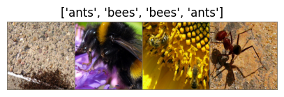
- We will train a classifier to distinguish between ants and bees.
- The data can be downloaded here: download link.
- There are two main transfer learning scenarios:
- Fine-tuning a ConvNet: instead of random initialization, we initialize the network with a pre-trained network, such as VGG trained on the ImageNet 1000 dataset. The rest of training looks the same as usual, although we often use a lower learning rate.
- ConvNet as a fixed feature extractor: here, we freeze all network weights except the final fully connected layer. The final fully connected layer is replaced with a new layer with random weights, and only this layer is trained. The advantage is very fast training, but several parts of the model do not adapt to the new target.
import os
import numpy as np
import time
import torch
import torchvision
import torch.nn as nn
from torch.utils.data import DataLoader
from torchvision.datasets import ImageFolder
from torchvision import models, transforms
import matplotlib.pyplot as plt

# Data augmentation and normalization for training
# Just normalization for validation
data_transforms = {
    'train': transforms.Compose([
        transforms.RandomResizedCrop(224),
        transforms.RandomHorizontalFlip(),
        transforms.ToTensor(),
        transforms.Normalize([0.485, 0.456, 0.406], [0.229, 0.224, 0.225])
    ]),
    'val': transforms.Compose([
        transforms.Resize(256),
        transforms.CenterCrop(224),
        transforms.ToTensor(),
        transforms.Normalize([0.485, 0.456, 0.406], [0.229, 0.224, 0.225])
    ]),
}

batch_size = 4
data_dir = './datasets/hymenoptera_data'
image_datasets = {x: ImageFolder(os.path.join(data_dir, x), data_transforms[x]) for x in ['train', 'val']}
dataloaders = {x: DataLoader(image_datasets[x], batch_size=batch_size,
                             shuffle=True, num_workers=4) for x in ['train', 'val']}
dataset_sizes = {x: len(image_datasets[x]) for x in ['train', 'val']}
class_names = image_datasets['train'].classes

device = torch.device("cuda:0" if torch.cuda.is_available() else "cpu")
print(device)cuda:0def imshow(inp, title=None):
"""Imshow for Tensor."""
inp = inp.numpy().transpose((1, 2, 0))
mean = np.array([0.485, 0.456, 0.406])
std = np.array([0.229, 0.224, 0.225])
inp = std * inp + mean
inp = np.clip(inp, 0, 1)
fig = plt.figure(figsize=(5, 8))
ax = fig.add_subplot(111)
ax.imshow(inp)
if title is not None:
ax.set_title(title)
ax.set_axis_off()
# Let’s visualize a few training images so as to understand the data augmentations.
# Get a batch of training data
inputs, classes = next(iter(dataloaders['train']))
# Make a grid from batch
out = torchvision.utils.make_grid(inputs)
imshow(out, title=[class_names[x] for x in classes])
Setting the .requires_grad Attribute of Model Parameters
- When we do feature extraction, the helper function below sets the
.requires_gradattribute of the model parameters toFalse. - By default, when we load a pre-trained model, all parameters have
.requires_grad=True. This is fine if we train from scratch or fine-tune the model. - However, if we do feature extraction and only want to compute gradients for the newly initialized layer, we want all other parameters to not require gradients.
def set_parameter_requires_grad(model, feature_extracting=False):
    # approach 1
    if feature_extracting:
        # frozen model
        model.requires_grad_(False)
    else:
        # fine-tuning
        model.requires_grad_(True)

    # approach 2
    if feature_extracting:
        # frozen model
        for param in model.parameters():
            param.requires_grad = False
    else:
        # fine-tuning
        for param in model.parameters():
            param.requires_grad = True
    # note: you can also mix between frozen layers and trainable layers, but you'll need a custom
    # function that loops over the model's layers and you specify which layers are frozen.
Initializing and Reshaping the Network
-
Recall that the last layer of a CNN model, usually an FC layer, has the same number of nodes as the number of output classes in the dataset.
-
Because all the following models were pre-trained on ImageNet, they all have an output layer of size 1000, with one node for each class.
-
Here, our goal is to reshape the last layer so that it has the same number of inputs as before, and the same number of outputs as the number of classes in our dataset.
-
During feature extraction, we only want to update the parameters of the last layer. In other words, we only want to update the parameters of the layer that we are reshaping.
-
Therefore, we do not need to compute gradients for parameters that we do not change. For efficiency, we set their
.requires_gradattribute toFalse. -
This is important because this attribute is set to
Trueby default. Then, when we initialize the new layer, its new parameters also have.requires_grad=Trueby default, so only the parameters of the new layer are updated. -
When we fine-tune, we can keep all
.required_gradvalues at the default value,True.
 Torchvision Pre-trained Models
- The
torchvision.modelssubpackage contains model definitions for different tasks, including image classification, pixel-level semantic segmentation, object detection, instance segmentation, person keypoint detection, video classification, and optical flow. - You can see everything available here: models and pre-trained weights.
- In code, you can use
torchvision.models.list\_modelsto view the list of all available models. - Example:
def initialize_model(model_name, num_classes, feature_extract, use_pretrained=True):
    # Initialize these variables which will be set in this if statement. Each of these
    #   variables is model specific.
    model_ft = None
    input_size = 0  # image size, e.g. (3, 224, 224)
    # new method from torchvision >= 0.13
    weigths = 'DEFAULT' if use_pretrained else None
    # to use other checkpoints than the default ones, check the model's available chekpoints here:
    # https://pytorch.org/vision/stable/models.html
    if model_name == "resnet":
        """ Resnet18
        """
        # new method from torchvision >= 0.13
        model_ft = models.resnet18(weights=weights)
        # old method for toechvision < 0.13
        # model_ft = models.resnet18(pretrained=use_pretrained)

        set_parameter_requires_grad(model_ft, feature_extract)
        num_ftrs = model_ft.fc.in_features
        model_ft.fc = nn.Linear(num_ftrs, num_classes) # replace the last FC layer
        input_size = 224

    elif model_name == "alexnet":
        """ Alexnet
        """
        # new method from torchvision >= 0.13
        model_ft = models.alexnet(weights=models)
        # old method for toechvision < 0.13
        # model_ft = models.alexnet(pretrained=use_pretrained)

        set_parameter_requires_grad(model_ft, feature_extract)
        num_ftrs = model_ft.classifier[6].in_features
        model_ft.classifier[6] = nn.Linear(num_ftrs, num_classes)
        input_size = 224

    elif model_name == "vgg":
        """ VGG16
        """
        # new method from torchvision >= 0.13
        model_ft = models.vgg16(weights=models.VGG16_Weights.DEFAULT)
        # old method for toechvision < 0.13
        # model_ft = models.vgg16(pretrained=use_pretrained)

        set_parameter_requires_grad(model_ft, feature_extract)
        num_ftrs = model_ft.classifier[6].in_features
        model_ft.classifier[6] = nn.Linear(num_ftrs, num_classes)
        input_size = 224

    elif model_name == "squeezenet":
        """ Squeezenet
        """
        # new method from torchvision >= 0.13
        model_ft = models.squeezenet1_0(weights=weights)
        # old method for torchvision < 0.13
        # model_ft = models.squeezenet1_0(pretrained=use_pretrained)

        set_parameter_requires_grad(model_ft, feature_extract)
        model_ft.classifier[1] = nn.Conv2d(512, num_classes, kernel_size=(1,1), stride=(1,1))
        model_ft.num_classes = num_classes
        input_size = 224

    elif model_name == "densenet":
        """ Densenet
        """
        # new method from torchvision >= 0.13
        model_ft = models.densenet121(weights=weights)
        # old method for torchvision < 0.13
        # model_ft = models.densenet121(pretrained=use_pretrained)

        set_parameter_requires_grad(model_ft, feature_extract)
        num_ftrs = model_ft.classifier.in_features
        model_ft.classifier = nn.Linear(num_ftrs, num_classes)
        input_size = 224

    else:
        raise NotImplementedError

    return model_ft, input_size
# Models to choose from [resnet, alexnet, vgg, squeezenet, densenet]
model_name = "vgg"
# Number of classes in the dataset
num_classes = 2
# Batch size for training (change depending on how much memory you have)
batch_size = 8
# Number of epochs to train for
num_epochs = 5
# Flag for feature extracting. When False, we fine-tune the whole model,
# when True we only update the reshaped layer params
feature_extract = True# Initialize the model for this run
model_ft, input_size = initialize_model(model_name, num_classes, feature_extract, use_pretrained=True)
# Print the model we just instantiated
print(model_ft)VGG(
(features): Sequential(
(0): Conv2d(3, 64, kernel_size=(3, 3), stride=(1, 1), padding=(1, 1))
(1): ReLU(inplace=True)
(2): Conv2d(64, 64, kernel_size=(3, 3), stride=(1, 1), padding=(1, 1))
(3): ReLU(inplace=True)
(4): MaxPool2d(kernel_size=2, stride=2, padding=0, dilation=1, ceil_mode=False)
(5): Conv2d(64, 128, kernel_size=(3, 3), stride=(1, 1), padding=(1, 1))
(6): ReLU(inplace=True)
(7): Conv2d(128, 128, kernel_size=(3, 3), stride=(1, 1), padding=(1, 1))
(8): ReLU(inplace=True)
(9): MaxPool2d(kernel_size=2, stride=2, padding=0, dilation=1, ceil_mode=False)
(10): Conv2d(128, 256, kernel_size=(3, 3), stride=(1, 1), padding=(1, 1))
(11): ReLU(inplace=True)
(12): Conv2d(256, 256, kernel_size=(3, 3), stride=(1, 1), padding=(1, 1))
(13): ReLU(inplace=True)
(14): Conv2d(256, 256, kernel_size=(3, 3), stride=(1, 1), padding=(1, 1))
(15): ReLU(inplace=True)
(16): MaxPool2d(kernel_size=2, stride=2, padding=0, dilation=1, ceil_mode=False)
(17): Conv2d(256, 512, kernel_size=(3, 3), stride=(1, 1), padding=(1, 1))
(18): ReLU(inplace=True)
(19): Conv2d(512, 512, kernel_size=(3, 3), stride=(1, 1), padding=(1, 1))
(20): ReLU(inplace=True)
(21): Conv2d(512, 512, kernel_size=(3, 3), stride=(1, 1), padding=(1, 1))
(22): ReLU(inplace=True)
(23): MaxPool2d(kernel_size=2, stride=2, padding=0, dilation=1, ceil_mode=False)
(24): Conv2d(512, 512, kernel_size=(3, 3), stride=(1, 1), padding=(1, 1))
(25): ReLU(inplace=True)
(26): Conv2d(512, 512, kernel_size=(3, 3), stride=(1, 1), padding=(1, 1))
(27): ReLU(inplace=True)
(28): Conv2d(512, 512, kernel_size=(3, 3), stride=(1, 1), padding=(1, 1))
(29): ReLU(inplace=True)
(30): MaxPool2d(kernel_size=2, stride=2, padding=0, dilation=1, ceil_mode=False)
)
(avgpool): AdaptiveAvgPool2d(output_size=(7, 7))
(classifier): Sequential(
(0): Linear(in_features=25088, out_features=4096, bias=True)
(1): ReLU(inplace=True)
(2): Dropout(p=0.5, inplace=False)
(3): Linear(in_features=4096, out_features=4096, bias=True)
(4): ReLU(inplace=True)
(5): Dropout(p=0.5, inplace=False)
(6): Linear(in_features=4096, out_features=2, bias=True)
)
)model_ft = model_ft.to(device)
# Gather the parameters to be optimized/updated in this run. If we are
# fine-tuning we will be updating all parameters. However, if we are
# doing feature extract method, we will only update the parameters
# that we have just initialized, i.e. the parameters with requires_grad
# is True.
params_to_update = model_ft.parameters()
print("Params to learn:")
if feature_extract:
params_to_update = [] # override the initial list definition above
for name,param in model_ft.named_parameters():
if param.requires_grad == True:
params_to_update.append(param)
print("\t",name)
else:
for name,param in model_ft.named_parameters():
if param.requires_grad == True:
print("\t",name)
# Observe that all parameters are being optimized
optimizer_ft = torch.optim.SGD(params_to_update, lr=0.001, momentum=0.9)Params to learn:
classifier.6.weight
classifier.6.biasimport copy
"""
Training function
"""
def train_model(model, dataloaders, criterion, optimizer, num_epochs=10):
since = time.time()
val_acc_history = []
best_model_wts = copy.deepcopy(model.state_dict())
best_acc = 0.0
for epoch in range(num_epochs):
print('Epoch {}/{}'.format(epoch, num_epochs - 1))
print('-' * 10)
# Each epoch has a training and validation phase
for phase in ['train', 'val']:
if phase == 'train':
model.train() # Set model to training mode
else:
model.eval() # Set model to evaluate mode
running_loss = 0.0
running_corrects = 0
# Iterate over data.
for inputs, labels in dataloaders[phase]:
inputs = inputs.to(device)
labels = labels.to(device)
# forward
# track history if only in train
with torch.set_grad_enabled(phase == 'train'):
# Get model outputs and calculate loss
outputs = model(inputs)
loss = criterion(outputs, labels)
_, preds = torch.max(outputs, 1)
# backward + optimize only if in training phase
if phase == 'train':
# zero the parameter gradients
optimizer.zero_grad()
loss.backward()
optimizer.step()
# statistics
running_loss += loss.item() * inputs.size(0)
running_corrects += torch.sum(preds == labels.data)
epoch_loss = running_loss / len(dataloaders[phase].dataset)
epoch_acc = running_corrects.double() / len(dataloaders[phase].dataset)
print('{} Loss: {:.4f} Acc: {:.4f}'.format(phase, epoch_loss, epoch_acc))
# deep copy the model
if phase == 'val' and epoch_acc > best_acc:
best_acc = epoch_acc
best_model_wts = copy.deepcopy(model.state_dict())
if phase == 'val':
val_acc_history.append(epoch_acc)
print()
time_elapsed = time.time() - since
print('Training complete in {:.0f}m {:.0f}s'.format(time_elapsed // 60, time_elapsed % 60))
print('Best val Acc: {:4f}'.format(best_acc))
# load best model weights
model.load_state_dict(best_model_wts)
return model, val_acc_history# Setup the loss fn
criterion = nn.CrossEntropyLoss()
# Train and evaluate
model_ft, hist = train_model(model_ft, dataloaders, criterion, optimizer_ft, num_epochs=num_epochs)Epoch 0/4
----------
train Loss: 0.3457 Acc: 0.8770
val Loss: 0.1964 Acc: 0.9346
Epoch 1/4
----------
train Loss: 0.2492 Acc: 0.9139
val Loss: 0.1017 Acc: 0.9739
Epoch 2/4
----------
train Loss: 0.2920 Acc: 0.9303
val Loss: 0.1045 Acc: 0.9673
Epoch 3/4
----------
train Loss: 0.1478 Acc: 0.9385
val Loss: 0.2151 Acc: 0.9216
Epoch 4/4
----------
train Loss: 0.2607 Acc: 0.9180
val Loss: 0.1252 Acc: 0.9477
Training complete in 0m 9s
Best val Acc: 0.973856 Pre-training in Natural Language Processing
- One of the biggest challenges in NLP is the shortage of labeled training data.
- Because NLP is a diverse field with many different tasks, most task-specific datasets contain only a few thousand or a few hundred thousand manually labeled training examples.
- As large companies such as Google and OpenAI have shown, modern deep-learning-based NLP models benefit from large amounts of data. They improve when trained on millions or billions of annotated training examples.
- Large pre-trained models trained on a large amount of unannotated text from the web can then be fine-tuned on small-data NLP tasks, such as question answering and sentiment analysis. This gives much higher accuracy than training from scratch on these datasets.
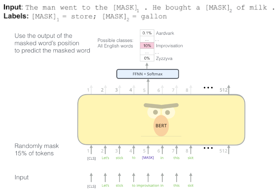
- Bidirectional Encoder Representations from Transformers (BERT), Google – BERT is a Transformer-based machine learning technique developed by Google for natural language processing (NLP) pre-training. The idea is to mask some words and then try to predict them. The original English BERT model has two general pre-trained versions:
- (1) The $BERT_{BASE}$ model: 12 layers, 768 hidden units, 12 heads, and 110M parameters.
- (2) The $BERT_{LARGE}$ model: 24 layers, 1024 hidden units, 16 heads, and 340M parameters.
- Both were trained on the BooksCorpus dataset with 800M words and the English Wikipedia with 2,500M words.
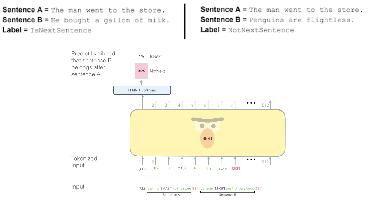
- BERT uses a simple technique to mask some words in the input, and then conditions each word bidirectionally to predict the masked words. At the same time, it learns relationships between sentences through a very simple pre-training task that can be generated from any text corpus: given two sentences A and B, is B the real next sentence after A in the corpus, or is it just a random sentence?
Pre-trained Models for NLP in PyTorch
- HuggingFace is a company that publishes many available pre-trained models. It also works with PyTorch: HuggingFace Transformers.
- Example using PyTorch
- Tutorial: fine-tuning Transformers for NLP tasks with PyTorch and HuggingFace.
 TorchTune Library – Fine-tuning and Experimenting with LLMs
- TorchTune is a native PyTorch library that makes it easy to write, fine-tune, and experiment with LLMs.
- It provides native PyTorch implementations of popular LLMs and supports checkpoints in several formats, including HuggingFace-format checkpoints.
- TorchTune on GitHub

 Credits
- Icons made by Becris from www.flaticon.com
- Icons from Icons8.com – https://icons8.com
- Datasets from Kaggle – https://www.kaggle.com/
- Jason Brownlee – Why Initialize a Neural Network with Random Weights?
- OpenAI – Deep Double Descent
- Tal Daniel