Learning Methods of Deep Learning

create by Deepfinder

Agenda

Learning from a Teacher: Supervised Learning
Seeing the Whole from Small Clues: Unsupervised Learning
Learning Without a Teacher: Self-supervised Learning
Learning Broadly from a Few Labels: Semi-supervised Learning
Distinguishing Similarities and Differences: Contrastive Learning
Learning by Analogy: Transfer Learning
Competing Against Each Other: Adversarial Learning
Strength in Numbers: Ensemble Learning
Different Paths to the Same Goal: Federated Learning
Learning Through Trial and Error: Reinforcement Learning
Learning by Asking: Active Learning
Learning How to Learn: Meta-Learning

Tutorial 05 – Distinguishing Similarities and Differences: Contrastive Learning

Contrastive Learning

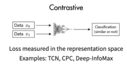
Contrastive learning is a way to define a task where a deep learning model learns to find things that are similar and things that are not similar. This is basically what classification does when labels are given.
As the name suggests, contrastive methods learn representations by comparing positive and negative examples.
With this method, we can train a machine learning model to classify similar and dissimilar images.

More formally, for any data point $x$, a contrastive method aims to learn an encoder $f$ such that:

$x^+$ is a data point similar to $x$. It is called a positive sample.
$x^−$ is a data point not similar to $x$. It is called a negative sample.
The score function measures the similarity between two features: $$score(f(x), f(x^+)) >> score(f(x), f(x^-))$$

Image Source
The most common loss function for implementing this scoring paradigm is the InfoNCE loss, which looks similar to softmax.

The denominator consists of one positive sample and $N−1$ negative samples.

But if we are in a self-supervised setting, how do we obtain negative samples?

InfoNCE loss in PyTorch

Contrastive Predictive Coding

Contrastive Predictive Coding (CPC) learns self-supervised representations by using a powerful autoregressive model to predict the future in a learned latent space.
The model uses a probabilistic contrastive loss. This encourages the latent space to capture information that is most useful for predicting future samples.

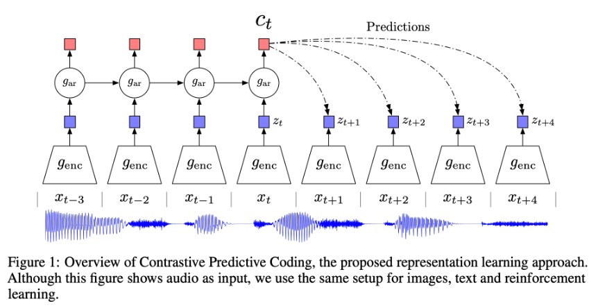
First, a nonlinear encoder $g_{enc}$ maps an input observation sequence $x_t$ to a sequence of latent representations $z_t = g_{enc}(x_t)$. The sequence may have a lower temporal resolution. The architecture of $g_{enc}$ usually depends on the data type, such as a CNN for images.
Next, an autoregressive model $g_{ar}$ summarizes all $z \leq t$ in the latent space and produces a context latent representation $c_t=g_{ar}(z \leq t)$.
The similarity function $f$ is modeled to preserve the mutual information between $x_{t+k}$ and $c_t$, as shown below: $$ f_k(x_{t+k}, c_t) = \exp(z_{t+k}^T W_k c_t) \propto \frac{p(x_{t+k} | c_t)}{p(x_{t+k})} $$

You can understand CPC (Contrastive Predictive Coding) in this way:

The encoder ( $g_{\mathrm{enc}}$ ) maps the input at each time step, such as text or another modality, to a latent vector representation $z_t$.
The autoregressive model ( $g_{\mathrm{ar}}$ ) aggregates semantics along the time dimension and outputs a context vector $c_t$. This vector represents the model’s understanding of all information up to the current time step.
During training:
- Choose a time step $t$. Use the context $c_t$ and the true future latent vector $z_{t+1}$ as a positive example.
- Use the context $c_t$ and latent vectors from other time steps or unrelated samples, $z_{\mathrm{neg}}$, as negative examples.
- Through a contrastive loss such as InfoNCE, the model learns to distinguish positive examples from negative examples. It pulls truly related time-step representations closer and pushes unrelated time-step representations farther apart.

The intuition is:

“Given the semantics of the past time steps, can the model correctly identify the real next time step?”
In a self-supervised framework, this encourages the model to learn predictive representations that are sensitive to the relationship between context and the future.

Therefore, “encoder + autoregressive model + InfoNCE contrastive loss” forms the basic idea of CPC. For text, you can remember it simply as:

First, “encode” each time step.

Then use “autoregression” to summarize the past.

Finally, use a “contrastive loss” to pull the correct next-step representation closer and push incorrect next-step representations farther away.

PyTorch code

Is the context prediction task in BERT a form of contrastive learning?

A Simple Framework for Contrastive Learning of Visual Representations

A Simple Framework for Contrastive Learning of Visual Representations (SimCLR) is a framework for contrastive learning of visual representations.
It learns representations by maximizing agreement between different augmented views of the same data example through a contrastive loss in the latent space.

How is a positive pair defined?

Random data augmentation: apply two random augmentations to the same original image $x$ to obtain two augmented images: $\tilde{x}_i \quad \text { and } \quad \tilde{x}_j$.
They come from the same image. They are just two views produced by augmentation operations such as cropping, color jittering, and blurring.
Called a “positive pair”: these two views are semantically the same because they come from the same original image. Therefore, $\left(\tilde{x}_i, \tilde{x}_j\right)$ is treated as a “positive pair”.
All positive pairs in a mini-batch: during training, a mini-batch containing $N$ original images is sampled. Two augmented views are generated for each original image. Therefore, the mini-batch finally contains $2 N$ “image views”. For each original image $x$, its two views form a positive pair.

Where do negative examples come from?

Explicit “negative examples” vs. implicit “negative examples”

Traditional contrastive learning methods often need to explicitly find different images as “negative examples”. For example, they may sample images from other classes to build negative examples. SimCLR proposes a very simple and effective method: there is no need to explicitly select negative examples. We can simply treat all other views in the mini-batch as negative examples for the current view.

Concrete definition

Suppose a mini-batch contains $N$ original images. It produces $2 N$ augmented views in total, with 2 views per image times $N$ images. If we focus on one positive pair $\left(\tilde{x}_i, \tilde{x}_j\right)$, then for $\tilde{x}_i$:

Its “positive example” is $\tilde{x}_j$, because both come from the same original image.
The remaining $2 N-2$ views in the mini-batch are treated as negative examples. These include augmented views of other images. The other member of $\tilde{x}_i$’s own pair is already counted as the positive example, so it is excluded.

Benefits

This greatly reduces the complexity of managing positive and negative examples. There is no need to maintain a large negative pool or mine negative examples online. We only need to compute the contrastive loss within one mini-batch and treat the other views as negative examples.

Image Source

For any augmented view in the mini-batch, when computing its loss, it “should” be similar only to its paired positive view and dissimilar to all other views. This naturally defines the distinction between positive and negative examples. By applying contrastive loss along the mini-batch dimension, SimCLR can learn highly discriminative visual representations without labels.

CLIP – Contrastive Language–Image Pre-training

CLIP is a neural network that efficiently learns visual concepts from natural language supervision.
CLIP can be applied to any visual classification benchmark in a zero-shot manner. We only need to provide the names of the visual categories to recognize.
Training data: text paired with images found on the internet.
Self-supervised task: given an image, predict which one among a set of randomly sampled text snippets is actually paired with the image in the dataset. This is similar to the matching paradigm introduced earlier.
Loss function: a scaled cross-entropy loss based on cosine similarity between pairs.
At inference time, we can classify photos of dogs and cats by checking whether the CLIP model predicts that the text description “a photo of a dog” or “a photo of a cat” is more likely to be paired with each image.
Official repository (PyTorch)
Colab example – interacting with CLIP and zero-shot classification
HuggingFace demos:
CLIP-ViT-Large
CLIPScore

# clip usage example
import torch
import clip
from PIL import Image

device = "cuda" if torch.cuda.is_available() else "cpu"
model, preprocess = clip.load("ViT-B/32", device=device)

image = preprocess(Image.open("CLIP.png")).unsqueeze(0).to(device)
text = clip.tokenize(["a diagram", "a dog", "a cat"]).to(device)

with torch.no_grad():
    image_features = model.encode_image(image)
    text_features = model.encode_text(text)

    logits_per_image, logits_per_text = model(image, text)
    probs = logits_per_image.softmax(dim=-1).cpu().numpy()

print("Label probs:", probs)  # prints: [[0.9927937  0.00421068 0.00299572]]

Credits

Icons made by Becris from www.flaticon.com
Icons from Icons8.com – https://icons8.com
Datasets from Kaggle – https://www.kaggle.com/
Jason Brownlee – Why Initialize a Neural Network with Random Weights?
OpenAI – Deep Double Descent
Tal Daniel