
Learning Methods of Deep Learning
create by Deepfinder
 Agenda
- Teacher and apprentice: Supervised Learning
- Seeing the whole from small clues: Unsupervised Learning
- Learning without a teacher: Self-supervised Learning
- From a few points to the whole picture: Semi-supervised Learning
- Distinguishing right from wrong: Contrastive Learning
- Learning by analogy: Transfer Learning
- Head-to-head: Adversarial Learning
- United effort: Ensemble Learning
- Different paths to the same goal: Federated Learning
- Perseverance: Reinforcement Learning
- Eager to learn: Active Learning
- Unifying all methods: Meta-Learning
Tutorial 04 – From a Few Points to the Whole Picture: Semi-supervised Learning
Semi-supervised learning is a method for training models when only a small part of the samples have human labels and most samples are unlabeled. It can still use all the data effectively, including both labeled and unlabeled data. It uses the information in labeled data from supervised learning. It also explores the hidden structure or distribution in unlabeled data, which can improve model performance.
Below we introduce the main common approaches and ideas in semi-supervised learning.
1. Self-Training / Pseudo-Labeling
Core idea
- Use the current model to generate “pseudo-labels” for unlabeled data. Then treat them as labeled data, add them to training, and update the model iteratively.
- The concrete process is: first train an initial model with a small amount of labeled data. Then let the model make predictions on unlabeled data. Add high-confidence predictions as pseudo-labels to the training set, and train the model again.
Representative methods
- Self-Training: the most basic method. Predict labels for unlabeled samples and filter out samples with low model confidence. Only keep high-confidence pseudo-labels and add them to the new training set.
- Pseudo-Labeling: a simple implementation proposed by Google Brain. The model labels unlabeled data by itself, and then uses these newly generated labels as true labels for training.
Advantages & limitations
- Advantages: simple to implement and easy to combine with other methods.
- Limitations: if the initial model has a large bias, the pseudo-label quality may be low. Wrong labels may “pollute” training and cause performance to degrade.
 If the model’s early predictions are biased, and we use wrong predictions as “true labels” for retraining, could the model become more and more wrong?
2. Consistency Regularization
Core idea
- Assumption: for the same unlabeled sample, the model output should stay consistent after different perturbations or augmentations. We use this consistency error as a regularization term. In other words, the predictions for different augmented views of the same data should be as similar as possible.
Concrete implementation
- In semi-supervised learning, there are usually two datasets:
- Labeled dataset $D_L$: it has fewer samples, but each sample has a label.
- Unlabeled dataset $D_U$: it has many samples, but no labels.
- For $D_L$, we usually use a supervised learning loss function, such as cross-entropy for classification:
$$
\mathcal{L}_{\text {supervised }}=\sum_{(x, y) \in D_L} \operatorname{CE}\left(f_\theta(x), y\right)
$$
Here, $f_\theta$ denotes the model, and CE denotes cross-entropy.
- For $D_U$, we do not have true labels. But we still want the model to have “stable outputs”. This is consistency regularization:
$$
\mathcal{L}_{\text {consistency }}=\sum_{x \in D_U} d\left(f_\theta\left(\operatorname{Aug}_1(x)\right), f_\theta\left(\operatorname{Aug}_2(x)\right)\right)
$$
-
$\mathrm{Aug}_1, \mathrm{Aug}_2$ are two random augmentation or perturbation methods applied to the same unlabeled sample.
-
$d(\cdot, \cdot)$ can be mean squared error, KL divergence, or another metric function. It measures the difference between the prediction distributions after the two augmentations.
-
We require the predictions of the two augmented views to be as similar as possible. This encourages the model to produce consistent outputs for “the same sample”.
-
Putting everything together, during training we take a weighted sum of the two losses above:
$$
\mathcal{L}_{\text {total }}=\mathcal{L}_{\text {supervised }}+\lambda \cdot \mathcal{L}_{\text {consistency }}
$$
- Here, $\lambda$ is a hyperparameter. It balances the relative weights of the supervised loss and the consistency loss.
- In this way, we use labeled data to provide supervised signals for class separation. We also use unlabeled data to provide a consistency regularization constraint, which improves the model’s discriminative ability and generalization ability.
Advantages & limitations
- Advantages: it can effectively use the distribution information in unlabeled data. It works especially well with data augmentation in computer vision.
- Limitations: the consistency constraint depends on suitable data augmentation or perturbation methods. Different tasks need different designs.
3. Generative Approaches
Core idea
- Learn a distribution model of the data, such as a variational autoencoder (VAE) or a GAN. During this process, use both labeled and unlabeled data, so the model can capture the data distribution and also distinguish different classes.
Representative methods
- VAE + classifier: use the latent space obtained by the VAE encoder both to reconstruct unlabeled samples and to help the classifier distinguish classes.
- Semi-Supervised GAN: in the GAN framework, introduce a discriminator that can distinguish both “the class of a real image” and “a generated image”. This allows the model to learn discriminative features with only a small number of labels.
Advantages & limitations
- Advantages: generative modeling can better explore the data distribution and has strong representation learning ability on unlabeled data.
- Limitations: stable training of GANs or VAEs, and the strategy for combining them with classification tasks, can be complex.
import os
import pickle
import torch
import random
import numpy as np
from torch.utils.data import Dataset, DataLoader
import torch.nn as nn
import torch.nn.functional as F
import torch.optim as optim

# ---------------------------
# 1. Set random seed and device
# ---------------------------

random.seed(42)
np.random.seed(42)
torch.manual_seed(42)

device = torch.device('cuda' if torch.cuda.is_available() else 'cpu')
print(f"Using device: {device}")

# ---------------------------
# 2. Load CIFAR-10 data
# ---------------------------

def load_cifar10_batch(file_path):
    """
    Load a single batch file and return images and labels.
    """
    with open(file_path, 'rb') as f:
        batch = pickle.load(f, encoding='bytes')
        images = batch[b'data']  # shape: (10000, 3072)
        labels = batch[b'labels'] if b'labels' in batch else batch[b'fine_labels']

        # Reshape images to (N, 3, 32, 32)
        images = images.reshape(-1, 3, 32, 32)
        images = images.astype(np.float32) / 255.0  # Normalize to [0,1]

        # Convert to Tensor
        images = torch.tensor(images)
        labels = torch.tensor(labels, dtype=torch.long)

    return images, labels

def load_cifar10_data(data_dir):
    """
    Load the full CIFAR-10 dataset and return training and test images and labels.
    """
    train_images = []
    train_labels = []

    # Load training batches
    for i in range(1, 6):
        batch_file = os.path.join(data_dir, f'data_batch_{i}')
        images, labels = load_cifar10_batch(batch_file)
        train_images.append(images)
        train_labels.append(labels)

    # Concatenate all training batches
    train_images = torch.cat(train_images, dim=0)  # shape: (50000, 3, 32, 32)
    train_labels = torch.cat(train_labels, dim=0)  # shape: (50000,)

    # Load test batch
    test_file = os.path.join(data_dir, 'test_batch')
    test_images, test_labels = load_cifar10_batch(test_file)  # shape: (10000, 3, 32, 32), (10000,)

    return train_images, train_labels, test_images, test_labels

# Specify the CIFAR-10 data directory
CIFAR10_DIR = 'datasets/cifar-10-batches-py'  # Change this according to the actual path

# Load data
train_images_all, train_labels_all, test_images_all, test_labels_all = load_cifar10_data(CIFAR10_DIR)

print(f"Number of training images: {train_images_all.shape[0]}")
print(f"Number of test images: {test_images_all.shape[0]}")
Using device: cuda
Number of training images: 50000
Number of test images: 10000
Partially labeled data
You will notice that all images in the dataset already have corresponding labels. If you train a model with all the data, then you will have a fully supervised model.
In the spirit of semi-supervised learning, we need to simulate a lack of labeled data. A simple way is to extract a small subset of images and their corresponding labels. Then you can pretend that everything else has no labels.
The following code extracts this “supervised” data subset. Note that all object classes have the same number of extracted samples. We recommend starting with only 1% of the dataset, so testing and debugging later code will be faster. Of course, you can increase this proportion later.
# ---------------------------
# 3. Split “labeled” and “unlabeled” data
# ---------------------------

NUM_LABELED_PER_CLASS = 50  # Number of labeled samples per class
NUM_CLASSES = 10

# Initialize counters
count_per_class = [0] * NUM_CLASSES

labeled_images = []
labeled_labels = []
unlabeled_images = []
unlabeled_labels = []

# Shuffle indices to ensure randomness
indices = list(range(len(train_images_all)))
random.shuffle(indices)

for idx in indices:
    img = train_images_all[idx]
    lbl = train_labels_all[idx].item()

    if count_per_class[lbl] < NUM_LABELED_PER_CLASS:
        labeled_images.append(img)
        labeled_labels.append(lbl)
        count_per_class[lbl] += 1
    else:
        unlabeled_images.append(img)
        unlabeled_labels.append(lbl)  # Labels still exist, but they will not be used later

print(f"Number of labeled data samples: {len(labeled_images)}")      # Expected: 10 * 50 = 500
print(f"Number of unlabeled data samples: {len(unlabeled_images)}")    # Expected: 50000 - 500 = 49500

# ---------------------------
# 4. Define PyTorch Dataset classes
# ---------------------------

class LabeledCIFARDataset(Dataset):
    def __init__(self, images, labels):
        """
        Labeled dataset
        """
        self.images = images
        self.labels = labels

    def __len__(self):
        return len(self.images)

    def __getitem__(self, idx):
        x = self.images[idx]
        y = self.labels[idx]
        return x, y

class UnlabeledCIFARDataset(Dataset):
    def __init__(self, images):
        """
        Unlabeled dataset
        """
        self.images = images

    def __len__(self):
        return len(self.images)

    def __getitem__(self, idx):
        x = self.images[idx]
        return x

class CIFARValDataset(Dataset):
    def __init__(self, images, labels):
        """
        Validation/test dataset
        """
        self.images = images
        self.labels = labels

    def __len__(self):
        return len(self.images)

    def __getitem__(self, idx):
        x = self.images[idx]
        y = self.labels[idx]
        return x, y

# ---------------------------
# 5. Create DataLoaders
# ---------------------------

BATCH_SIZE = 64

# Labeled DataLoader
labeled_dataset = LabeledCIFARDataset(labeled_images, labeled_labels)
labeled_loader = DataLoader(
    labeled_dataset,
    batch_size=BATCH_SIZE,
    shuffle=True
)

# Unlabeled DataLoader
unlabeled_dataset = UnlabeledCIFARDataset(unlabeled_images)
unlabeled_loader = DataLoader(
    unlabeled_dataset,
    batch_size=BATCH_SIZE,
    shuffle=True
)

# Validation/test DataLoader
val_dataset = CIFARValDataset(test_images_all, test_labels_all)
val_loader = DataLoader(
    val_dataset,
    batch_size=BATCH_SIZE,
    shuffle=False
)

print(f"Number of labeled data batches: {len(labeled_loader)}")      # 500 / 64 ≈ 8
print(f"Number of unlabeled data batches: {len(unlabeled_loader)}")    # 49500 / 64 ≈ 774
print(f"Number of validation/test data batches: {len(val_loader)}")      # 10000 / 64 ≈ 157
Number of labeled data samples: 500
Number of unlabeled data samples: 49500
Number of labeled data batches: 8
Number of unlabeled data batches: 774
Number of validation/test data batches: 157Define the model architecture
Now that the data is ready, let us turn to the model architecture. Remember that our goal is not to get the best performance from the data we have. Instead, we focus on learning how to implement semi-supervised techniques. With this in mind, we will study a simple toy model that can be built from scratch.
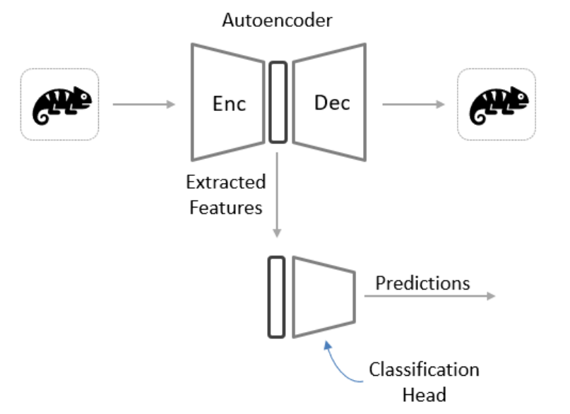
You should now be familiar with several semi-supervised techniques. Here, we use VAE + classifier as an example. It can be trained for two different tasks.
# ---------------------------
# 6. Define the model (VAE + classifier)
# ---------------------------

class Encoder(nn.Module):
    def __init__(self, latent_dim=32):
        super(Encoder, self).__init__()
        self.conv1 = nn.Conv2d(3, 16, 3, stride=2, padding=1)  # [B, 16, 16, 16]
        self.conv2 = nn.Conv2d(16, 32, 3, stride=2, padding=1) # [B, 32, 8, 8]
        self.fc = nn.Linear(32*8*8, 128)
        self.mu_layer = nn.Linear(128, latent_dim)
        self.logvar_layer = nn.Linear(128, latent_dim)

    def forward(self, x):
        h = F.relu(self.conv1(x))  # [B, 16, 16, 16]
        h = F.relu(self.conv2(h))  # [B, 32, 8, 8]
        h = h.view(h.size(0), -1)  # [B, 32*8*8]
        h = F.relu(self.fc(h))     # [B, 128]
        mu = self.mu_layer(h)      # [B, latent_dim]
        logvar = self.logvar_layer(h)  # [B, latent_dim]
        return mu, logvar

class Decoder(nn.Module):
    def __init__(self, latent_dim=32):
        super(Decoder, self).__init__()
        self.fc = nn.Linear(latent_dim, 32*8*8)
        self.deconv1 = nn.ConvTranspose2d(32, 16, 4, stride=2, padding=1)  # [B,16,16,16]
        self.deconv2 = nn.ConvTranspose2d(16, 3, 4, stride=2, padding=1)   # [B,3,32,32]

    def forward(self, z):
        h = F.relu(self.fc(z))              # [B, 32*8*8]
        h = h.view(h.size(0), 32, 8, 8)     # [B, 32, 8, 8]
        h = F.relu(self.deconv1(h))         # [B, 16, 16, 16]
        x_recon = torch.sigmoid(self.deconv2(h))  # [B, 3, 32, 32]
        return x_recon

class Classifier(nn.Module):
    def __init__(self, latent_dim=32, num_classes=10):
        super(Classifier, self).__init__()
        self.fc1 = nn.Linear(latent_dim, 64)
        self.fc2 = nn.Linear(64, num_classes)

    def forward(self, z):
        h = F.relu(self.fc1(z))  # [B, 64]
        logits = self.fc2(h)     # [B, num_classes]
        return logits

class VAE_Classifier(nn.Module):
    def __init__(self, latent_dim=32, num_classes=10):
        super(VAE_Classifier, self).__init__()
        self.encoder = Encoder(latent_dim)
        self.decoder = Decoder(latent_dim)
        self.classifier = Classifier(latent_dim, num_classes)

    def reparameterize(self, mu, logvar):
        std = torch.exp(0.5 * logvar)    # [B, latent_dim]
        eps = torch.randn_like(std)      # [B, latent_dim]
        return mu + eps * std            # [B, latent_dim]

    def forward_vae(self, x):
        mu, logvar = self.encoder(x)             # [B, latent_dim], [B, latent_dim]
        z = self.reparameterize(mu, logvar)      # [B, latent_dim]
        x_recon = self.decoder(z)                # [B, 3, 32, 32]
        return x_recon, mu, logvar, z

    def forward_classifier(self, x):
        mu, logvar = self.encoder(x)             # [B, latent_dim], [B, latent_dim]
        logits = self.classifier(mu)             # [B, num_classes]
        return logits

# Instantiate the model
latent_dim = 32
num_classes = 10
model = VAE_Classifier(latent_dim=latent_dim, num_classes=num_classes).to(device)
3. The “two losses” in the training stage
- 3.1 Train the VAE (unlabeled data can be used)
When training on unlabeled data, you only need the VAE reconstruction loss + KL divergence:
$$
\mathcal{L}_{\mathrm{VAE}}=|x-\hat{x}|^2(\text { or } \mathrm{BCE})+\mathrm{KL}\left[q_\phi(z \mid x) | p(z)\right]
$$
- Reconstruction loss: $|x-\hat{x}|^2$ or binary cross-entropy (BCE), and other metrics. It makes the decoder output $\hat{x}$ as similar as possible to the original image $x$.
- KL divergence: it makes the encoder’s latent distribution $q_\phi(z \mid x)$ close to the prior $p(z)$, which is usually $\mathcal{N}(0, I)$.
On unlabeled data, we do not calculate classification loss because there are no labels. But we can still learn latent representations through VAE reconstruction.
- 3.2 Train the classifier (labeled data is needed)
When training on labeled data, we update both the VAE and the classifier, because the classifier uses the encoder output:
$$
\mathcal{L}_{\text {Classifier }}=\text { CrossEntropy }(\text { logits }, y)
$$
where:
- logits = classifier(encoder(x)) (or reparameterized $z$).
- $y$ is the true class label of the image ($0 \sim 9$).
This part only exists for “labeled data”.
- 3.3 Total loss
Putting them together, you can update the model on labeled and unlabeled batches either at the same time or alternately.
def vae_loss_function(x, x_recon, mu, logvar):
    # x: [B, 3, 32, 32]
    # x_recon: [B, 3, 32, 32]
    # mu, logvar: [B, latent_dim]

    # 1) Reconstruction loss - use BCE
    recon_loss = F.binary_cross_entropy(x_recon, x, reduction='sum') / x.size(0)
    # Or use mean() and then adjust the balance as needed

    # 2) KL divergence
    # KL = 0.5 * sum( exp(logvar) + mu^2 - 1 - logvar )
    kl_divergence = 0.5 * torch.mean(torch.sum(torch.exp(logvar) + mu**2 - 1. - logvar, dim=1))

    return recon_loss + kl_divergence, recon_loss, kl_divergence

def classifier_loss_function(logits, y):
    return F.cross_entropy(logits, y)

# ---------------------------
# 8. Define the validation function
# ---------------------------

def evaluate_on_valset(model, val_loader):
    """
    Evaluate classification accuracy on the validation set.
    """
    model.eval()
    correct = 0
    total = 0
    with torch.no_grad():
        for x_val, y_val in val_loader:
            x_val = x_val.to(device)
            y_val = y_val.to(device)

            logits = model.forward_classifier(x_val)  # [B, num_classes]
            preds = torch.argmax(logits, dim=1)       # [B]
            correct += (preds == y_val).sum().item()
            total += y_val.size(0)
    acc = correct / total
    return acc
# ---------------------------
# 9. Implement baseline and semi-supervised training
# ---------------------------
def train_baseline(model, labeled_loader, val_loader, epochs=10, lr=1e-3):
"""
Baseline training: use only labeled data to train the model.
"""
optimizer = optim.Adam(model.parameters(), lr=lr)
for epoch in range(epochs):
model.train()
total_loss = 0.0
total_clf = 0.0
for x_labeled, y_labeled in labeled_loader:
x_labeled = x_labeled.to(device)
y_labeled = y_labeled.to(device)
optimizer.zero_grad()
# Classifier forward pass
logits = model.forward_classifier(x_labeled)
clf_loss = classifier_loss_function(logits, y_labeled)
# Backpropagation and optimization
clf_loss.backward()
optimizer.step()
total_loss += clf_loss.item()
total_clf += clf_loss.item()
# Calculate average loss
avg_loss = total_loss / len(labeled_loader)
avg_clf = total_clf / len(labeled_loader)
# Evaluate on validation set
val_acc = evaluate_on_valset(model, val_loader)
print(f"[Baseline] Epoch {epoch+1}/{epochs}, Loss: {avg_loss:.4f}, Clf: {avg_clf:.4f}, Val Acc: {val_acc:.4f}")
return model
def train_semi_supervised(model, labeled_loader, unlabeled_loader, val_loader, epochs=10, lr=1e-3, lambda_unsupervised=1.0, confidence_threshold=0.8):
"""
Semi-supervised training: use labeled and unlabeled data at the same time.
"""
optimizer = optim.Adam(model.parameters(), lr=lr)
for epoch in range(epochs):
model.train()
total_loss = 0.0
total_recon = 0.0
total_kl = 0.0
total_clf = 0.0
total_unsupervised = 0.0
# a) Training on labeled data
for x_labeled, y_labeled in labeled_loader:
x_labeled = x_labeled.to(device)
y_labeled = y_labeled.to(device)
optimizer.zero_grad()
# VAE forward pass
x_recon, mu, logvar, z = model.forward_vae(x_labeled)
vae_loss, recon_loss, kl_div = vae_loss_function(x_labeled, x_recon, mu, logvar)
# Classifier forward pass
logits = model.forward_classifier(x_labeled)
clf_loss = classifier_loss_function(logits, y_labeled)
# Combine losses
total_batch_loss = vae_loss + clf_loss
total_batch_loss.backward()
optimizer.step()
total_loss += total_batch_loss.item()
total_recon += recon_loss.item()
total_kl += kl_div.item()
total_clf += clf_loss.item()
# b) Training on unlabeled data (pseudo-labels)
for x_unlabeled in unlabeled_loader:
x_unlabeled = x_unlabeled.to(device)
optimizer.zero_grad()
# Generate pseudo-labels
logits = model.forward_classifier(x_unlabeled)
probs = torch.softmax(logits, dim=-1)
max_probs, pseudo_labels = torch.max(probs, dim=-1)
# Use only high-confidence pseudo-labels
high_confidence_mask = max_probs > confidence_threshold
if high_confidence_mask.sum() > 0:
pseudo_labels = pseudo_labels[high_confidence_mask]
x_unlabeled = x_unlabeled[high_confidence_mask]
# Calculate classification loss for unlabeled data
clf_loss = classifier_loss_function(logits[high_confidence_mask], pseudo_labels)
# Total loss = unlabeled data loss + labeled data loss
total_unsupervised_loss = lambda_unsupervised * clf_loss
total_unsupervised_loss.backward()
optimizer.step()
total_unsupervised += total_unsupervised_loss.item()
# Calculate average losses
avg_loss = total_loss / len(labeled_loader)
avg_recon = total_recon / len(labeled_loader)
avg_kl = total_kl / len(labeled_loader)
avg_clf = total_clf / len(labeled_loader)
avg_unsupervised = total_unsupervised / len(unlabeled_loader)
# Evaluate on validation set
val_acc = evaluate_on_valset(model, val_loader)
print(f"[Semi-Supervised] Epoch {epoch+1}/{epochs}, Loss: {avg_loss:.4f}, Clf: {avg_clf:.4f}, Unsupervised: {avg_unsupervised:.4f}, Val Acc: {val_acc:.4f}")
return model
# ---------------------------
# 10. Run training and compare
# ---------------------------

def main():
    # Instantiate two independent models
    model_baseline = VAE_Classifier(latent_dim=latent_dim, num_classes=num_classes).to(device)
    model_semi = VAE_Classifier(latent_dim=latent_dim, num_classes=num_classes).to(device)

    # Define training parameters
    epochs = 10
    learning_rate = 1e-2

    print("Start baseline training (labeled data only)...")
    model_baseline = train_baseline(model_baseline, labeled_loader, val_loader, epochs=epochs, lr=learning_rate)

    print("\nStart semi-supervised training (labeled + unlabeled data)...")
    model_semi = train_semi_supervised(model_semi, labeled_loader, unlabeled_loader, val_loader, epochs=epochs, lr=learning_rate)

    # Final evaluation comparison
    baseline_acc = evaluate_on_valset(model_baseline, val_loader)
    semi_acc = evaluate_on_valset(model_semi, val_loader)

    print(f"\nFinal comparison results:\n  Baseline accuracy = {baseline_acc:.4f}\n  Semi-supervised accuracy = {semi_acc:.4f}")

if __name__ == "__main__":
    main()
Start baseline training (labeled data only)...
[Baseline] Epoch 1/10, Loss: 2.3153, Clf: 2.3153, Val Acc: 0.1000
[Baseline] Epoch 2/10, Loss: 2.3001, Clf: 2.3001, Val Acc: 0.1632
[Baseline] Epoch 3/10, Loss: 2.2466, Clf: 2.2466, Val Acc: 0.1284
[Baseline] Epoch 4/10, Loss: 2.2630, Clf: 2.2630, Val Acc: 0.1401
[Baseline] Epoch 5/10, Loss: 2.2094, Clf: 2.2094, Val Acc: 0.1573
[Baseline] Epoch 6/10, Loss: 2.1534, Clf: 2.1534, Val Acc: 0.1925
[Baseline] Epoch 7/10, Loss: 2.1225, Clf: 2.1225, Val Acc: 0.2331
[Baseline] Epoch 8/10, Loss: 2.0578, Clf: 2.0578, Val Acc: 0.2203
[Baseline] Epoch 9/10, Loss: 2.0038, Clf: 2.0038, Val Acc: 0.2675
[Baseline] Epoch 10/10, Loss: 1.8889, Clf: 1.8889, Val Acc: 0.2509
Start semi-supervised training (labeled + unlabeled data)...
[Semi-Supervised] Epoch 1/10, Loss: 2130.3845, Clf: 2.3115, Unsupervised: 0.0000, Val Acc: 0.0872
[Semi-Supervised] Epoch 2/10, Loss: 2125.7730, Clf: 2.2873, Unsupervised: 0.0000, Val Acc: 0.1113
[Semi-Supervised] Epoch 3/10, Loss: 2106.7699, Clf: 2.2789, Unsupervised: 0.0000, Val Acc: 0.1629
[Semi-Supervised] Epoch 4/10, Loss: 2088.1254, Clf: 2.2613, Unsupervised: 0.0000, Val Acc: 0.1784
[Semi-Supervised] Epoch 5/10, Loss: 2069.3262, Clf: 2.2282, Unsupervised: 0.0000, Val Acc: 0.2065
[Semi-Supervised] Epoch 6/10, Loss: 2087.0404, Clf: 2.1865, Unsupervised: 0.0000, Val Acc: 0.1421
[Semi-Supervised] Epoch 7/10, Loss: 2071.9022, Clf: 2.1797, Unsupervised: 0.0000, Val Acc: 0.1959
[Semi-Supervised] Epoch 8/10, Loss: 2049.9933, Clf: 2.1584, Unsupervised: 0.0000, Val Acc: 0.2161
[Semi-Supervised] Epoch 9/10, Loss: 2037.8330, Clf: 2.1724, Unsupervised: 0.0000, Val Acc: 0.1703
[Semi-Supervised] Epoch 10/10, Loss: 2030.8822, Clf: 2.1445, Unsupervised: 0.0000, Val Acc: 0.2203
Final comparison results:
Baseline accuracy = 0.2509
Semi-supervised accuracy = 0.2203The final comparison shows that the baseline model has an accuracy of 0.2509, while the semi-supervised model has an accuracy of 0.2203. Note that this project is only a demo. Its main purpose is to explain the basic principles and workflow of semi-supervised training, not to pursue the best final accuracy. The effect of semi-supervised training usually depends on a large amount of data, careful parameter tuning, and suitable model design. In real applications, semi-supervised learning can improve model performance by using unlabeled data, but this process requires repeated experiments and adjustments. Therefore, the current result does not represent the full potential of semi-supervised learning. It only provides a starting point for further exploration and optimization.
 Credits
- Icons made by Becris from www.flaticon.com
- Icons from Icons8.com – https://icons8.com
- Datasets from Kaggle – https://www.kaggle.com/
- Jason Brownlee – Why Initialize a Neural Network with Random Weights?
- OpenAI – Deep Double Descent
- Tal Daniel