
 Deep Learning
create by Deepfinder
 Agenda
- Learning from a Teacher: Supervised Learning
- Seeing the Pattern from Small Clues: Unsupervised Learning
- Learning Without a Teacher: Self-supervised Learning
- Learning from a Few Labels: Semi-supervised Learning
- Learning by Comparison: Contrastive Learning
- Generalizing from One Case to Many: Transfer Learning
- Learning Through Opposition: Adversarial Learning
- Strength in Numbers: Ensemble Learning
- Different Paths to One Goal: Federated Learning
- Persistence Through Trial and Error: Reinforcement Learning
- Eager to Learn: Active Learning
- Unifying the Methods: Meta-Learning
 Basic Principles of Reinforcement Learning
In today’s fast-moving technical world, reinforcement learning (RL) is an important branch of machine learning. It is quickly becoming a key topic for understanding artificial intelligence (AI) and machine learning. Compared with traditional machine learning methods, reinforcement learning uniquely focuses on learning how to make optimal decisions from feedback from the environment. This method has great potential for complex problems that require continuous decision making, so it has attracted a lot of attention in recent years. Reinforcement learning gives machines the ability to learn how to make decisions in complex environments, and its applications are changing the world.
- It plays an important role in many fields, such as:
- Robotics: helping robots learn complex tasks such as walking or grasping.
- Games: AI players learn how to beat human opponents in complex games.
- Autonomous vehicles: one of the core technologies that helps vehicles react quickly in complex road environments.
- Personalized recommendation systems: dynamic adjustment based on user behavior and preferences.
- As technology continues to improve and innovate, reinforcement learning may have wider application scenarios in the future:
- Smart grids: optimizing energy distribution and consumption for more efficient power management.
- Healthcare: helping doctors make more accurate diagnosis and treatment decisions.
- Smart cities: optimizing traffic flow and public services in urban planning and management.
- Finance: making more accurate predictions and decisions in investment and risk management.
 Basic Concepts in Reinforcement Learning
- Agent (Agent): In the reinforcement learning (RL) framework, an agent is an entity that can observe and interact with an environment. It makes decisions by taking actions and receiving feedback from the environment, usually as reward signals. The goal of the agent is to learn how to choose actions that maximize long-term cumulative reward.
- Environment (Environment): The environment is the external system in which the agent operates. It defines the boundaries and rules of the problem. In reinforcement learning, the environment receives the agent’s actions and responds with a new state and a reward. This determines the agent’s learning process.
- State (State, s): A state is a description or observation of the environment at a specific moment. It is usually treated as the information set used by the agent to make decisions. The state must contain enough information about the environment so that the agent can choose actions effectively.
- State Probability Density Function (State Probability Density Function): This is a mathematical function that describes the probability distribution over possible next states, given the current state and the agent’s action. It is a core element for understanding and predicting environment dynamics.
- State Value Function (State Value Function, V(s)): The state value function estimates the expected return that can be obtained by starting from state s and following policy π. It is used to evaluate the long-term performance of starting from a given state and following a specific policy.
- Policy (Policy, π): A policy maps states to actions. In a deterministic policy, it defines the action the agent will take in a given state. In a stochastic policy, it defines the probability of choosing each possible action in a given state.
- Action (Action, a): An action is any operation that the agent can choose in a given state. Actions affect the state of the agent and the cumulative return it receives through feedback from the environment.
- Action Probability Density Function (Action Probability Density Function): This function describes the probability distribution for selecting each possible action under a given state and policy. In continuous action spaces, it defines the probability density over all possible actions.
- Action-Value Function (Action-Value Function, Q(s,a)): The action-value function, or Q-function, estimates the expected return obtained by starting from state s, taking action a, and then following policy π. It is key for evaluating the long-term performance of a specific action in a specific state under a specific policy.
- Reward (Reward): A reward is the immediate feedback given by the environment after the agent takes an action. It is the key signal that guides learning and action selection in reinforcement learning.
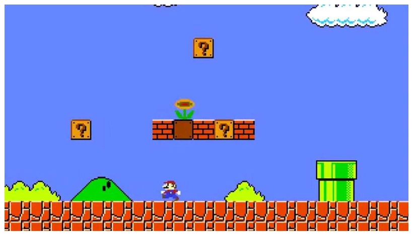
- Cumulative Reward (Cumulative Reward): Cumulative reward is the sum of rewards obtained by the agent from the current time step to a future time step or to the end of an episode. It is the main optimization objective in reinforcement learning. The agent learns and makes decisions to maximize this cumulative value.
- Exploration (Exploration): Exploration is the process in which the agent tries unknown or less-tried actions. The goal is to discover more valuable choices or information and improve the decision policy.
- Exploitation (Exploitation): Exploitation means choosing actions that are already known to produce high rewards. In exploitation, the agent relies on existing knowledge instead of seeking new information.
- Trajectory (Trajectory): In reinforcement learning, a trajectory is a sequence of states (s), actions (a), and rewards (r) experienced by the agent while interacting with the environment.
Understanding Randomness in Reinforcement Learning
In reinforcement learning (RL), randomness, or uncertainty, is a core concept. It appears in many places, including environment dynamics, the agent’s policy, the learning process, and reward signals. Understanding and handling this randomness is essential for designing effective RL algorithms. The main sources of randomness are described below:
- Randomness in the environment
- Randomness in state transitions: In most reinforcement learning problems, the state transition of the environment can be stochastic. When an agent takes an action in a state, it may move to several different next states with certain probabilities.
- Randomness in rewards: In some RL problems, even under the same state and action, the reward may be different each time. This reflects uncertainty or noise in the environment.
- Randomness in the policy:
- Exploration and exploitation: In reinforcement learning, the agent needs to balance exploration, which tries new or rare actions to obtain more information, and exploitation, which chooses the best action based on existing knowledge. Exploration often involves randomness. For example, the agent may randomly choose an action with a certain probability instead of always choosing the action that currently looks best.
- Stochastic policy: In some algorithms, such as policy gradient methods, the policy itself may be stochastic. This means that even in the same state, the agent may choose different actions with certain probabilities.
- Randomness in the learning process:
- Initialization: The performance of reinforcement learning algorithms may be affected by initial conditions, such as random initialization of neural network weights. In addition, when experience replay is used, as in DQN, randomly sampling from the replay buffer also introduces randomness.
- Stochastic Gradient Descent (SGD): In gradient-based learning methods, the gradient estimate is usually based on randomly selected samples instead of the full dataset. This also introduces randomness.
- Randomness in reinforcement learning is a double-edged sword:
- On one hand, it increases the complexity and difficulty of learning.
- On the other hand, proper randomness helps the agent explore the environment and avoid local optima.
- Therefore, understanding and using randomness properly is key to designing efficient reinforcement learning systems.
 Value-based Deep Reinforcement Learning (DQN)
To understand DQN, we first need to understand the Q-value. The Q-value is a function. Q(s, a) represents the expected reward from taking action a in state s.
Intuitively, the Q-value tells the agent which actions are more beneficial in the long run。
The goal of Q-learning is to find the optimal Q-value function, so that the agent can choose the best action by looking at Q-values.
How can we find the Q-function?
The appeal of deep learning is that when a problem is difficult to solve explicitly, we can let a neural network learn it.
In DQN, we use a deep neural network to predict Q-values. The input to the network is the state, and the output is the Q-value for each action.
- Imagine a robot, or agent, playing a game.
- Its goal is to get as many points, or rewards, as possible. Each scene in the game can be treated as a state. The robot can take different actions, such as moving left or moving right.
- In DQN, we let the robot learn by itself. The robot tries different actions and observes which actions bring higher scores.
- In traditional reinforcement learning, the robot has a scoreboard, or Q-table. It records the possible score for taking different actions in each scene, or state. This is the idea behind algorithms such as Sarsa.
- When the game becomes very complex, the scoreboard, or Q-table, becomes extremely large. The robot cannot remember all this information.
- In DQN, we use a neural network to help the robot estimate the scores on this board, namely the Q-values. The neural network tries to predict the score, or Q-value, obtained by taking a specific action in a specific state.
This raises a question: How can we make the neural network predict Q-values that are as close as possible to the true Q-values?Note that because the environment is complex and uncertain, these Q-values usually cannot be computed directly. They must be estimated and approximated gradually through interaction with the environment.The Bellman equation and temporal-difference learning are the keys to solving this problem.
Bellman Equation and Temporal-Difference Learning (TD-Learning)
- The Bellman equation is a core concept in reinforcement learning.
- The Bellman equation is based on the Markov Decision Process (MDP). It provides a recursive way to compute the current state value or action value while considering future rewards.
- The idea of recursion is to break a large problem into similar smaller problems.
- Here, the Bellman equation decomposes a long-term sequential decision problem into a one-step decision problem plus the remaining sequential decision problem. For the action-value function $Q(s, a)$, the Bellman equation can be written as:
$$
Q(s, a)=\mathbb{E}\left[R_{t+1}+\gamma \max _{a^{\prime}} Q\left(S_{t+1}, a^{\prime}\right) \mid S_t=s, A_t=a\right]
$$
Here, $\mathbb{E}[\cdot]$ denotes expectation, $R_{t+1}$ is the reward, and $\gamma$ is the discount factor, which measures the present value of future rewards. There are several key points:
- Immediate reward $R_{t+1}$: the reward the agent receives immediately after taking action $a$ in state $s$.
- Discounted future reward $\gamma \max _{d^{\prime}} Q\left(S_{t+1}, a^{\prime}\right)$: the discounted future return that the agent expects to obtain by taking the best action $a^{\prime}$ in the next state $S_{t+1}$. Here, $\gamma$, the discount factor, reduces the importance of future rewards compared with immediate rewards. This is intuitive. In real life, the expected value of receiving one hundred yuan ten years later is much smaller than receiving it immediately.
- Expectation $\mathbb{E}[\cdot]$: Because of uncertainty in the environment or randomness in the policy, the Bellman equation uses expectation to combine all possible next states and rewards. This ensures that the agent’s decision considers all possible future scenarios.
In the Bellman equation, the expectation $\mathbb{E}[\cdot]$ is the statistical average over the environment dynamics, that is, the transition from state $s$ through action $a$ to the next state $s^{\prime}$ and the reward $R_{t+1}$.
Accurately computing this expectation usually requires a complete model of the environment, including transition probabilities and the reward function. In many practical applications, this model is unknown or difficult to obtain precisely.
The main reasons are:
- Uncertainty in the environment
- A large state space
- A large action space
- Unknown model dynamics
These factors make it impractical or computationally infeasible to directly compute the expectation in the Bellman equation. Therefore, we use Temporal-Difference (TD) learning to estimate this value.
Specifically, TD learning simplifies the Bellman equation. It does not compute the full expectation. Instead, it uses the current estimate and the reward from the next state, or next few states, to update the value estimate. The update rule can be written as:
$$
Q\left(S_t, A_t\right) \leftarrow Q\left(S_t, A_t\right)+\alpha\left[R_{t+1}+\gamma \max _{a^{\prime}} Q\left(S_{t+1}, a^{\prime}\right)-Q\left(S_t, A_t\right)\right]
$$
Here:
- $-\alpha$ is the learning rate.
- $-R_{t+1}+\gamma \max _{a^{\prime}} Q\left(S_{t+1}, a^{\prime}\right)$ is the TD target, which represents an estimate of the value of the next state. This estimate is more accurate than directly estimating the next-state value because the current reward $R_{t+1}$ has already been observed.
- This is like estimating your arrival time at school after you have already reached a shop on the way. That estimate is more accurate than estimating the whole trip when you just left home, because the time from home to the shop has already been observed.
- How do we obtain the TD target?
- In deep reinforcement learning, such as DQN, a neural network is used to approximate the Q-function. The input is the state, and possibly the action. The output is the Q-value estimate for that state and action.
- Therefore, at any time, the value of the next state is estimated by the neural network based on its current parameters.
- In practice, this TD target is the label we use when training the neural network.
- $-R_{t+1}+\gamma \max _{a^{\prime}} Q\left(S_{t+1}, a^{\prime}\right)-Q\left(S_t, A_t\right)$ is the TD error. It is the difference between the current reward plus the discounted estimated value of the next state and the estimated value of the current state. We denote it as $\delta_t$.
- The basic idea of updating the $\mathrm{Q}$ value is:
- If the reward obtained for a state-action pair $\left(S_t, A_t\right)$ is larger than we expected, we should increase the $Q$ value of that state-action pair.
- Conversely, if the reward is smaller than expected, we should decrease the $Q$ value of that state-action pair.
- Therefore, the $Q$-value update formula in TD learning is:
$$
Q\left(S_t, A_t\right) \leftarrow Q\left(S_t, A_t\right)+\alpha \times \delta_t
$$
- Here, $\alpha$ is the learning rate. It determines how much we change the $\mathrm{Q}$ value at each update.
- If $\delta_t$ is positive, meaning the actual reward plus the future-reward estimate is higher than the current $Q$-value estimate, we increase $Q\left(S_t, A_t\right)$.
- If $\delta_t$ is negative, meaning the actual reward plus the future-reward estimate is lower than the current $\mathrm{Q}$-value estimate, we decrease $Q\left(S_t, A_t\right)$.
In this way, TD learning continuously adjusts its estimate of the value of each state-action pair, so it can better adapt to and learn the dynamics of the environment.Note that the update of the $Q$ value is not exactly the same as the loss function in supervised learning.
The $Q$-value update is more like an iterative value-estimation process. Through repeated correction based on the TD error, the predicted $Q$ value becomes closer to the true, or optimal, $Q$ value.
In each training step, the target $Q$ value from the TD update plays a role similar to a ground-truth label in supervised learning,but this “label” is itself being learned and adjusted. It is not a fixed ground-truth label like in supervised learning.
Training the Neural Network
- How do we train this neural network to predict Q-values?
- The first step in training the neural network is data collection.
- In reinforcement learning, the data usually consists of states, actions, rewards, and next states obtained while the agent interacts with the environment.
- These data are stored in an experience replay buffer for later training.
- Next comes sampling. Training the neural network involves randomly sampling a batch of examples from the replay buffer. This helps reduce correlation between samples and lowers the variance of training.
- For each sampled example, we compute the loss using the TD target and the current prediction of the network. The goal is to minimize the gap between the predicted Q-value and the TD target. The formula is:
$$
\operatorname{LossMSE}=\frac{1}{N} \sum_{i=1}^N\left(y_i-Q\left(s_i, a_i ; \theta\right)\right)^2
$$
where:
- $-N$ is the number of samples.
- $-y_i$ is the TD target value of the $i$-th sample, computed from the Bellman equation.
- $-Q\left(s_i, a_i ; \theta\right)$ is the Q-value predicted by the neural network for state $s_i$ and action $a_i$ under the current parameters $\theta$.
During training, we minimize MSE through gradient descent. This adjusts the network parameters $\theta$ so that the predicted $\mathrm{Q}$ value $Q(s, a ; \theta)$ approaches the TD target $y$, reducing the error between the network output and the expected output.
The whole training process is iterative. It continues until the desired performance standard is reached or the planned training period is completed.
During this process, we must maintain a balance between exploration and exploitation. The agent should use the current policy to maximize immediate reward, but it should also keep exploring new policies to discover behavior patterns that may produce higher long-term returns.
Evaluation Network and Target Network
- $R_{t+1}+\gamma \max _{a^{\prime}} Q\left(S_{t+1}, a^{\prime}\right)$ is the TD target.
- In DQN, a neural network is used to approximate the $\mathrm{Q}$ function. The network input is the state, and possibly the action. The output is the $\mathrm{Q}$-value estimate for that state and action.
- Therefore, at any time, the next-state value $Q\left(S_{t+1}, a^{\prime}\right)$ is actually estimated by the neural network based on its current parameters.
- This is a bootstrapping method, and using a single network to estimate $Q$ values and compute TD targets can create a “chasing its own tail” problem. The $Q$-value updates may become too frequent and too large.
- In this situation, the network is trained against a continuously changing target, so convergence is difficult, and the training process may become unstable and oscillatory.
- To solve this problem, DQN (Deep Q-Networks) and its variants usually use two neural networks: an evaluation network and a target network.
The evaluation network, also called the policy network, is used to estimate the value function in real time. In other words, this network predicts Q-values based on the current state and action. During learning, the parameters of this network are continuously updated to reflect the latest learning results.
The target network has the same structure as the evaluation network, but its parameters are updated less frequently. Its main role is to provide a relatively stable Q-value estimate when computing the temporal-difference target. This TD target is usually used to compute the loss function and perform gradient descent.Because the target network is updated later than the evaluation network, it provides a more stable learning target. This helps reduce the variance introduced by each update and makes training smoother. The separate target network can also reduce overfitting to some extent. Because it does not immediately reflect the newest learning results, it prevents the evaluation network from over-adapting to recent experiences and ignoring long-term strategy.
Note that the target network parameters are not updated at every iteration. Usually, they are copied from the evaluation network after a fixed number of time steps or training cycles. This update interval is a hyperparameter and should be adjusted for the specific application and task.
Exploration and Exploitation
The epsilon-greedy strategy is a basic reinforcement learning strategy used to balance exploration and exploitation. Its basic principle is:
- Choose a random action with probability epsilon (exploration).
- Choose the current best action with probability 1 – epsilon (exploitation).
By adjusting epsilon, we can control the agent’s exploration and exploitation behavior:
- Early in training, epsilon is high, so the agent explores more and tries different actions.
- Later in training, epsilon is low, so the agent uses more of what it has learned and chooses the best action.
Exponential decayWe use exponential decay to update epsilon, so epsilon gradually decreases from its initial value to its final value. This gives a smooth transition in the agent’s behavior:
- Early in training, the agent mainly explores so that it can better understand the environment.
- As training continues, the agent gradually reduces exploration and uses the learned knowledge more for decision making.
import matplotlib.pyplot as plt
import numpy as np

# Parameter definitions
epsilon_start = 1.0
epsilon_end = 0.01
epsilon_decay = 500
sample_count = np.arange(0, 2000)  # 2000 sampling steps

# Compute the epsilon value at each sampling point
epsilon_values = epsilon_end + (epsilon_start - epsilon_end) * np.exp(-1. * sample_count / epsilon_decay)

# Plot the epsilon value curve
plt.plot(sample_count, epsilon_values)
plt.xlabel('Sample Count')
plt.ylabel('Epsilon Value')
plt.title('Epsilon Decay Over Time')
plt.grid(True)
plt.show()
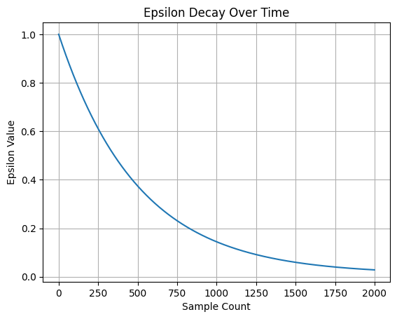
This dynamic strategy for adjusting exploration and exploitation helps the agent fully explore the environment early on and use the learned policy later. It improves training effectiveness and efficiency.
 Gym Library
- Gym is an open-source toolkit provided by OpenAI for developing and comparing reinforcement learning algorithms.
- It provides a set of standardized environments. These environments cover many types of problems and make it easier for researchers and developers to develop, test, and compare algorithms.
- The Gym library supports not only classic control and game problems, but also more complex tasks. For example:
- CartPole-v1: the classic pole-balancing problem.
- MountainCar-v0: a car needs to climb to the top of a hill.
- Acrobot-v1: a two-link robot needs to swing up to a target height.
- Pong-v0: the Pong game.
- Breakout-v0: the brick-breaking game.
- SpaceInvaders-v0: the Space Invaders game.
- LunarLander-v2: lunar lander.
- BipedalWalker-v2: bipedal robot walking.
- Humanoid-v2: simulated humanoid robot.
- Ant-v2: quadruped robot.
- FetchReach-v1: Fetch robot control task.
Detailed documentation and the environment list for the Gym library can be found on its official website: Gym Documentation
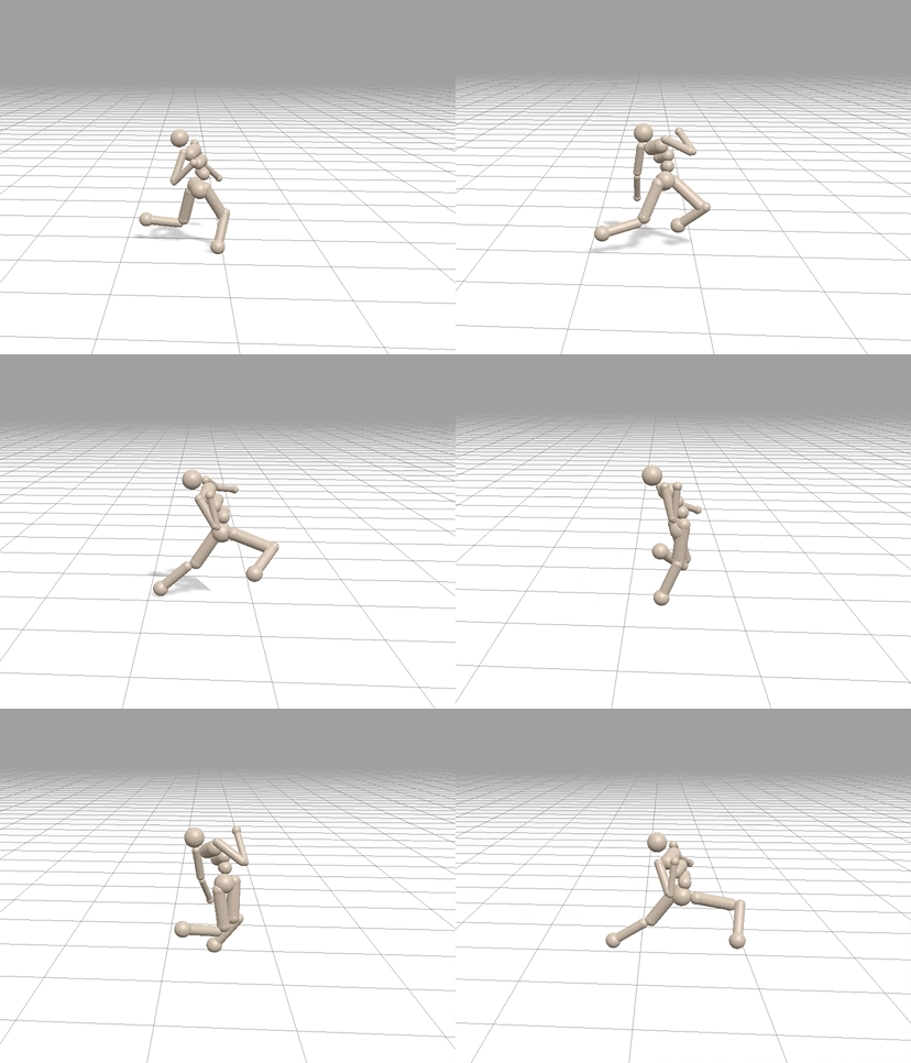
A Humanoid example is shown below:
A cart_pole example is shown below:
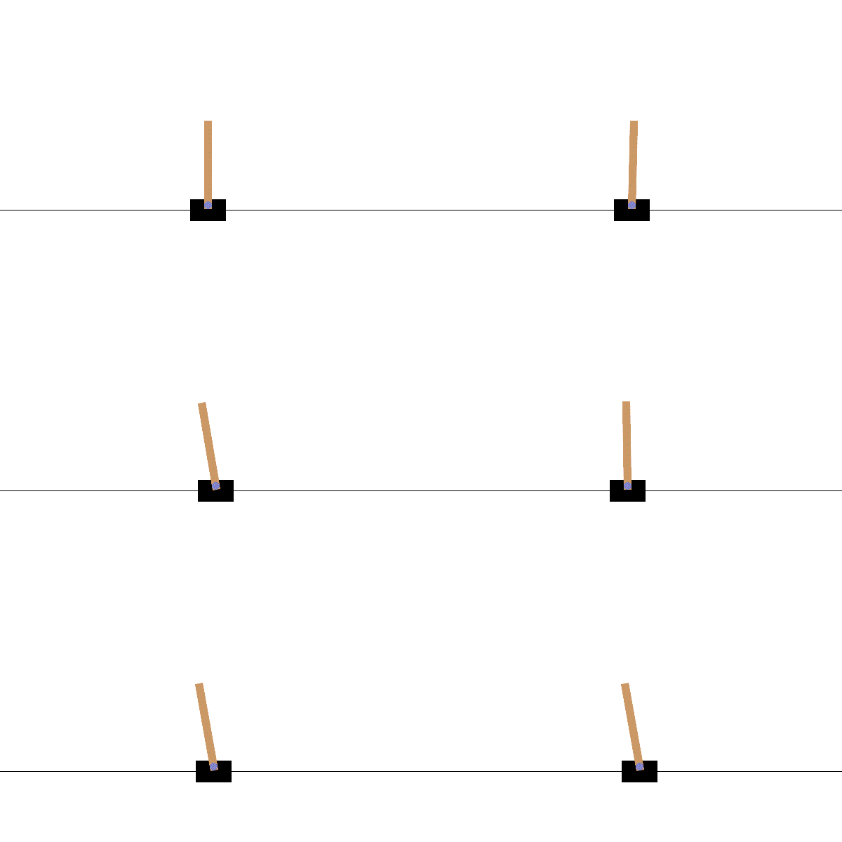
The code example in this project is also based on this game environment.
 Example Code: Value-based Reinforcement Learning
import torch
import torch.nn as nn
import torch.optim as optim
import torch.nn.functional as F
import numpy as np
import random
import math
import gym

# Define the replay buffer class for storing experiences
class ReplayBuffer:
    # Initialization method: define buffer capacity and position
    def __init__(self, capacity):
        self.buffer = []
        self.capacity = capacity
        self.position = 0

    # Add an experience to the buffer
    def push(self, transition):
        if len(self.buffer) < self.capacity:
            self.buffer.append(None)
        self.buffer[self.position] = transition
        self.position = (self.position + 1) % self.capacity

    # Randomly sample a batch of experiences from the buffer
    def sample(self, batch_size):
        batch = random.sample(self.buffer, batch_size)
        state, action, reward, next_state, done = map(np.stack, zip(*batch))
        return state, action, reward, next_state, done

    # Return the current size of the buffer
    def __len__(self):
        return len(self.buffer)

# Define the policy network class
class PolicyNetwork(nn.Module):

    def __init__(self, n_states, n_actions):
        super(PolicyNetwork, self).__init__()
        self.fc1 = nn.Linear(n_states, 128)
        self.fc2 = nn.Linear(128, n_actions)

    def forward(self, x):
        x = F.relu(self.fc1(x))
        x = self.fc2(x)
        return x

# Define the Deep Q-Network class
class DQN:
    # Initialization method: define related parameters and networks
    def __init__(self, model, memory, cfg):
        self.n_actions = cfg['n_actions']  # number of actions
        self.device = torch.device(cfg['device'])  # device (CPU or GPU)
        self.gamma = cfg['gamma']  # discount factor
        self.sample_count = 0  # sample count
        self.epsilon = cfg['epsilon_start']  # initial epsilon value
        self.epsilon_start = cfg['epsilon_start']  # initial epsilon value
        self.epsilon_end = cfg['epsilon_end']  # final epsilon value
        self.epsilon_decay = cfg['epsilon_decay']  # epsilon decay rate
        self.batch_size = cfg['batch_size']  # batch size
        self.policy_net = model.to(self.device)  # policy network
        self.target_net = model.to(self.device)  # target network
        # Initialize target network weights to match the policy network
        for target_param, param in zip(self.target_net.parameters(), self.policy_net.parameters()):
            target_param.data.copy_(param.data)
        self.optimizer = optim.Adam(self.policy_net.parameters(), lr=cfg['lr'])  # optimizer
        self.memory = memory  # replay buffer

    # Sample an action using the epsilon-greedy strategy
    def sample_action(self, state):
        self.sample_count += 1  # Increase the sample count
        # Update epsilon with exponential decay
        self.epsilon = self.epsilon_end + (self.epsilon_start - self.epsilon_end) * \
            math.exp(-1. * self.sample_count / self.epsilon_decay)
        if random.random() > self.epsilon:  # Choose the greedy policy
            with torch.no_grad():
                state = torch.tensor(state, device=self.device, dtype=torch.float32).unsqueeze(dim=0)
                q_values = self.policy_net(state)  # Compute Q-values
                action = q_values.max(1)[1].item()  # Choose the action with the largest Q-value
        else:  # Randomly choose an action
            action = random.randrange(self.n_actions)
        return action  # Return the action

    # Predict an action for the test phase
    @torch.no_grad()
    def predict_action(self, state):
        state = torch.tensor(state, device=self.device, dtype=torch.float32).unsqueeze(dim=0)
        q_values = self.policy_net(state)  # Compute Q-values
        action = q_values.max(1)[1].item()  # Choose the action with the largest Q-value
        return action  # Return the action

    # Update the network
    def update(self):
        if len(self.memory) < self.batch_size:  # If the buffer does not contain enough experiences for one batch
            return
        # Sample a batch of experiences from the buffer
        state_batch, action_batch, reward_batch, next_state_batch, done_batch = self.memory.sample(self.batch_size)
        # Convert to tensors
        state_batch = torch.tensor(np.array(state_batch), device=self.device, dtype=torch.float)
        action_batch = torch.tensor(action_batch, device=self.device).unsqueeze(1)
        reward_batch = torch.tensor(reward_batch, device=self.device, dtype=torch.float)
        next_state_batch = torch.tensor(np.array(next_state_batch), device=self.device, dtype=torch.float)
        done_batch = torch.tensor(np.float32(done_batch), device=self.device)
        # Compute current Q-values
        q_values = self.policy_net(state_batch).gather(dim=1, index=action_batch)
        # Compute Q-values for the next state
        next_q_values = self.target_net(next_state_batch).max(1)[0].detach()
        # Compute expected Q-values
        expected_q_values = reward_batch + self.gamma * next_q_values * (1 - done_batch)
        # Compute the loss
        loss = nn.MSELoss()(q_values, expected_q_values.unsqueeze(1))
        self.optimizer.zero_grad()  # Clear gradients
        loss.backward()  # Backpropagation
        # Gradient clipping
        for param in self.policy_net.parameters():
            param.grad.data.clamp_(-1, 1)
        self.optimizer.step()  # Update network parameters

# Environment and agent configuration function
def env_agent_config(cfg):
    env = gym.make(cfg['env_name'])  # Create the environment
    n_states = env.observation_space.shape[0]  # state-space dimension
    n_actions = env.action_space.n  # action-space dimension
    memory = ReplayBuffer(cfg['memory_capacity'])  # Create the replay buffer
    agent = DQN(PolicyNetwork(n_states, n_actions), memory, cfg)  # Create the DQN agent
    return env, agent  # Return the environment and agent

# Training function
def train(cfg, env, agent):
    print("Start training!")
    rewards = []  # Store rewards for each episode
    steps = []  # Store steps for each episode
    for i_ep in range(cfg['train_eps']):
        ep_reward = 0  # Initialize episode reward
        ep_step = 0  # Initialize episode steps
        state, _ = env.reset()  # Reset the environment and get the initial state
        for _ in range(cfg['ep_max_steps']):
            ep_step += 1
            action = agent.sample_action(state)  # Sample an action
            next_state, reward, done, truncated, info = env.step(action)  # Execute the action
            done = done or truncated
            agent.memory.push((state, action, reward, next_state, done))  # Store the experience in the buffer
            state = next_state  # Update the state
            agent.update()  # Update the evaluation network
            ep_reward += reward  # Accumulate reward
            if done:  # If the episode ends
                break
        if (i_ep + 1) % cfg['target_update'] == 0:  # Update the target network every fixed number of episodes
            agent.target_net.load_state_dict(agent.policy_net.state_dict())
        steps.append(ep_step)  # Record steps
        rewards.append(ep_reward)  # Record reward
        if (i_ep + 1) % 10 == 0:
            print(f"episode:{i_ep + 1}/{cfg['train_eps']},reward:{ep_reward:.2f},Epislon:{agent.epsilon:.3f}")
    print("Training complete!")
    env.close()  # Close the environment
    return {'rewards': rewards}  # Return reward records

# Testing function
def test(cfg, env, agent):
    print("Start testing!")
    rewards = []  # Store rewards for each episode
    steps = []  # Store steps for each episode
    for i_ep in range(cfg['test_eps']):
        ep_reward = 0  # Initialize episode reward
        ep_step = 0  # Initialize episode steps
        state, _ = env.reset()  # Reset the environment and get the initial state
        done = False  # Initialize the done flag
        while not done and ep_step < cfg['ep_max_steps']:
            ep_step += 1
            action = agent.predict_action(state)  # Predict an action
            next_state, reward, done, truncated, info = env.step(action)  # Execute the action
            done = done or truncated
            state = next_state  # Update the state
            ep_reward += reward  # Accumulate reward
            if done:
                print(f"episode {i_ep + 1} completed in {ep_step} steps")
        steps.append(ep_step)  # Record steps
        rewards.append(ep_reward)  # Record reward
        print(f"episode:{i_ep + 1}/{cfg['test_eps']},reward:{ep_reward:.2f}")
    print("Testing complete")
    env.close()  # Close the environment
    return {'rewards': rewards}  # Return reward records

# Function for getting configuration parameters
def get_args():
    return {
        'env_name': 'CartPole-v1',  # environment name
        'n_actions': 2,  # number of actions
        'device': 'cpu',  # device (CPU)
        'gamma': 0.99,  # discount factor
        'epsilon_start': 1.0,  # initial epsilon value
        'epsilon_end': 0.01,  # final epsilon value
        'epsilon_decay': 500,  # epsilon decay rate
        'batch_size': 64,  # batch size
        'lr': 0.001,  # learning rate
        'memory_capacity': 10000,  # buffer capacity
        'train_eps': 100,  # number of training episodes
        'test_eps': 100,  # number of test episodes
        'ep_max_steps': 200,  # maximum steps per episode
        'target_update': 10,  # target network update frequency
        'seed': 42  # random seed
    }

# Function for plotting the reward curve
def plot_rewards(rewards, cfg, tag="train"):
    import matplotlib.pyplot as plt
    plt.plot(rewards)  # Plot the reward curve
    plt.title(f'{tag} Rewards')  # Set the title
    plt.show()  # Show the image

# Get parameters
cfg = get_args()
# Train
env, agent = env_agent_config(cfg)
res_dic = train(cfg, env, agent)

# Plot the training reward curve
plot_rewards(res_dic['rewards'], cfg, tag="train")

# Test
res_dic = test(cfg, env, agent)

# Plot the test reward curve
plot_rewards(res_dic['rewards'], cfg, tag="test")
Start training!

/home/arwin/anaconda3/envs/dt/lib/python3.8/site-packages/gym/utils/passive\_env\_checker.py:233: DeprecationWarning: np.bool8 is a deprecated alias for np.bool\_. (Deprecated NumPy 1.24) if not isinstance(terminated, (bool, np.bool8)): Episode: 10/100, reward: 11.00, Epsilon: 0.586 Episode: 20/100, reward: 16.00, Epsilon: 0.401 Episode: 30/100, reward: 20.00, Epsilon: 0.290 Episode: 40/100, reward: 46.00, Epsilon: 0.152 Episode: 50/100, reward: 60.00, Epsilon: 0.059 Episode: 60/100, reward: 100.00, Epsilon: 0.027 Episode: 70/100, reward: 138.00, Epsilon: 0.014 Episode: 80/100, reward: 162.00, Epsilon: 0.010 Episode: 90/100, reward: 200.00, Epsilon: 0.010 Episode: 100/100, reward: 200.00, Epsilon: 0.010 Training complete!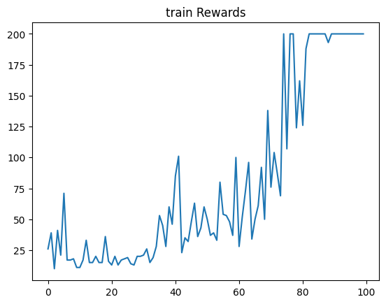
Start testing!
Episode 1 completed in 190 steps
Episode: 1/100, reward: 190.00
Episode: 2/100, reward: 200.00
Episode: 3/100, reward: 200.00
Episode 4 completed in 175 steps
Episode: 4/100, reward: 175.00
Episode 5 completed in 199 steps
Episode: 5/100, reward: 199.00
Episode 6 completed in 175 steps
Episode: 6/100, reward: 175.00
Episode: 7/100, reward: 200.00
Episode: 8/100, reward: 200.00
Episode: 9/100, reward: 200.00
Episode: 10/100, reward: 200.00
Episode: 11/100, reward: 200.00
Episode 12 completed in 188 steps
Episode: 12/100, reward: 188.00
Episode: 13/100, reward: 200.00
Episode: 14/100, reward: 200.00
Episode 15 completed in 197 steps
Episode: 15/100, reward: 197.00
Episode: 16/100, reward: 200.00
Episode: 17/100, reward: 200.00
Episode: 18/100, reward: 200.00
Episode: 19/100, reward: 200.00
Episode: 20/100, reward: 200.00
Episode 21 completed in 184 steps
Episode: 21/100, reward: 184.00
Episode: 22/100, reward: 200.00
Episode 23 completed in 187 steps
Episode: 23/100, reward: 187.00
Episode: 24/100, reward: 200.00
Episode 25 completed in 194 steps
Episode: 25/100, reward: 194.00
Episode: 26/100, reward: 200.00
Episode: 27/100, reward: 200.00
Episode 28 completed in 196 steps
Episode: 28/100, reward: 196.00
Episode: 29/100, reward: 200.00
Episode 30 completed in 199 steps
Episode: 30/100, reward: 199.00
Episode: 31/100, reward: 200.00
Episode: 32/100, reward: 200.00
Episode: 33/100, reward: 200.00
Episode 34 completed in 188 steps
Episode: 34/100, reward: 188.00
Episode 35 completed in 190 steps
Episode: 35/100, reward: 190.00
Episode: 36/100, reward: 200.00
Episode: 37/100, reward: 200.00
Episode: 38/100, reward: 200.00
Episode 39 completed in 192 steps
Episode: 39/100, reward: 192.00
Episode 40 completed in 191 steps
Episode: 40/100, reward: 191.00
Episode: 41/100, reward: 200.00
Episode 42 completed in 185 steps
Episode: 42/100, reward: 185.00
Episode: 43/100, reward: 200.00
Episode 44 completed in 184 steps
Episode: 44/100, reward: 184.00
Episode: 45/100, reward: 200.00
Episode 46 completed in 192 steps
Episode: 46/100, reward: 192.00
Episode: 47/100, reward: 200.00
Episode: 48/100, reward: 200.00
Episode: 49/100, reward: 200.00
Episode: 50/100, reward: 200.00
Episode: 51/100, reward: 200.00
Episode: 52/100, reward: 200.00
Episode: 53/100, reward: 200.00
Episode 54 completed in 194 steps
Episode: 54/100, reward: 194.00
Episode 55 completed in 181 steps
Episode: 55/100, reward: 181.00
Episode: 56/100, reward: 200.00
Episode: 57/100, reward: 200.00
Episode 58 completed in 185 steps
Episode: 58/100, reward: 185.00
Episode: 59/100, reward: 200.00
Episode 60 completed in 177 steps
Episode: 60/100, reward: 177.00
Episode 61 completed in 176 steps
Episode: 61/100, reward: 176.00
Episode: 62/100, reward: 200.00
Episode: 63/100, reward: 200.00
Episode: 64/100, reward: 200.00
Episode: 65/100, reward: 200.00
Episode: 66/100, reward: 200.00
Episode 67 completed in 185 steps
Episode: 67/100, reward: 185.00
Episode 68 completed in 200 steps
Episode: 68/100, reward: 200.00
Episode: 69/100, reward: 200.00
Episode: 70/100, reward: 200.00
Episode: 71/100, reward: 200.00
Episode 72 completed in 185 steps
Episode: 72/100, reward: 185.00
Episode: 73/100, reward: 200.00
Episode: 74/100, reward: 200.00
Episode: 75/100, reward: 200.00
Episode: 76/100, reward: 200.00
Episode: 77/100, reward: 200.00
Episode 78 completed in 191 steps
Episode: 78/100, reward: 191.00
Episode 79 completed in 173 steps
Episode: 79/100, reward: 173.00
Episode 80 completed in 188 steps
Episode: 80/100, reward: 188.00
Episode: 81/100, reward: 200.00
Episode: 82/100, reward: 200.00
Episode: 83/100, reward: 200.00
Episode: 84/100, reward: 200.00
Episode: 85/100, reward: 200.00
Episode 86 completed in 192 steps
Episode: 86/100, reward: 192.00
Episode: 87/100, reward: 200.00
Episode: 88/100, reward: 200.00
Episode 89 completed in 190 steps
Episode: 89/100, reward: 190.00
Episode 90 completed in 180 steps
Episode: 90/100, reward: 180.00
Episode: 91/100, reward: 200.00
Episode 92 completed in 197 steps
Episode: 92/100, reward: 197.00
Episode 93 completed in 195 steps
Episode: 93/100, reward: 195.00
Episode: 94/100, reward: 200.00
Episode: 95/100, reward: 200.00
Episode 96 completed in 189 steps
Episode: 96/100, reward: 189.00
Episode 97 completed in 192 steps
Episode: 97/100, reward: 192.00
Episode: 98/100, reward: 200.00
Episode: 99/100, reward: 200.00
Episode: 100/100, reward: 200.00
Testing complete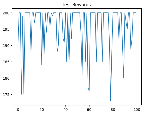
 Policy-based Deep Reinforcement Learning (Policy-based model)
- Imagine that you are teaching a robot how to walk.
- In policy-based reinforcement learning, you directly guide the robot on how to act at each step. This guidance is implemented through a probabilistic model, namely the policy function.
- The policy function considers the current environment, that is, the current state of the robot, and outputs the probability of each possible action. The robot chooses actions according to these probabilities.
- Therefore, in each state, the robot has clear probabilistic guidance for deciding what to do next.
- The key advantage of this method is that it can handle more complex and diverse action choices, such as choosing suitable force and direction in a continuous action space.
By contrast, in value-based reinforcement learning methods such as DQN, we do not directly tell the robot what to do at each step. Instead, we give it a scoring system: for each possible action, DQN evaluates the expected return, namely the Q-value. The robot’s task is to choose the action with the highest expected return at each step. This is like giving each possible step a score instead of telling the robot exactly how to move, and letting it find the highest-scoring step by itself. This method works very well in discrete action spaces because it is easy to compare and select the best option from a finite set of actions.
Now, if the action space becomes very large or continuous — imagine asking a robot to learn how to run at any speed and in any direction — value-based methods become complex and inefficient. For every possible action, we would need to compute an expected return and choose the best one. In a continuous action space, the number of possible actions is infinite, so finding the best action becomes very difficult.
Policy-based methods handle this situation more naturally. They do not compute a separate value for every possible action. Instead, they directly generate an action probability distribution from the current state. This lets the robot choose actions smoothly in a continuous action space rather than selecting from a small finite set.
Policy Gradient Optimization
- Policy-based reinforcement learning directly optimizes the policy itself, instead of indirectly deriving a policy from Q-values as in DQN.
- The policy is usually represented by a neural network. The input is the state, and the output is the probability of taking each possible action in that state.
- Policy gradient methods directly maximize the expected cumulative return by adjusting the parameters of the policy network.
- Among them, the REINFORCE algorithm is a classic policy gradient method.
- In REINFORCE, the policy network guides action selection, and then the network parameters are adjusted according to the actual return obtained.
- In short, if an action leads to a positive return, we increase the probability of choosing that action in the future. If it leads to a negative return, we decrease the probability of choosing it.
- The detailed algorithm steps are:
- Initialize the policy model: The policy is usually represented by a parameterized model, such as a neural network. The network outputs the probability of each available action based on the input state.
- Generate one or more episodes: At each iteration, use the current policy to run one or more complete trajectories in the environment until a terminal state is reached. Each trajectory is a sequence of states, actions, and returns.
- Compute returns: For each step in a trajectory, compute the cumulative return from the current state to the end of the trajectory. This cumulative return is usually a discounted sum of future returns, where the discount factor γ determines the weight of future returns.
- Policy gradient update: For each step in the trajectory, adjust the parameters of the policy model to increase the probability of choosing the action that was actually taken in the given state. This adjustment follows the policy gradient and is usually implemented with gradient ascent. The policy gradient is given by the product of the cumulative return at each step and the gradient of the action probability. Repeat these steps until the policy converges or reaches a performance target.
The basic form of the policy gradient can be written as:
$$
\nabla_\theta J(\theta)=\mathbb{E}\left[\sum_{t=0}^T G_t \cdot \nabla_\theta \log \pi_\theta\left(a_t \mid s_t\right)\right]
$$
Intuitively, we can explain this formula as follows:
- Expected return: $J(\theta)$ is the expected return under policy $\pi_\theta$. Our goal is to adjust $\theta$ to maximize $J(\theta)$.
- Gradient ascent: Because we want to maximize $J(\theta)$, we adjust $\theta$ in the direction of the gradient $\nabla_\theta J(\theta)$. If the gradient is positive in a certain direction, increasing $\theta$ in that direction will increase the expected return.
- Log probability of the policy: $\log \pi_\theta\left(a_t \mid s_t\right)$ is the natural logarithm of the policy probability of choosing action $a_t$ in state $s_t$. The logarithm makes gradient computation more stable and efficient.
- Gradient $\nabla_\theta \log \pi_\theta\left(a_t \mid s_t\right)$: This term shows how sensitive the policy probability is to the parameter $\theta$. Intuitively, it tells us how a small change in $\theta$ affects the probability of choosing action $a_t$ in state $s_t$.
- Cumulative return $G_t$: This is the cumulative discounted return from time $t$ to the end of the trajectory. Using $G_t$ ensures that action selection considers not only immediate reward, but also long-term impact. Through $G_t$, policy gradient methods can encourage actions that may have low immediate reward but good long-term effects.
- Expectation: The outer expectation $\mathbb{E}$ means that this gradient is the average gradient over all possible trajectories. Since directly computing this full expectation is usually infeasible, in practice we estimate it by sampling one or more trajectories from the current policy.
 Why multiply the gradient of the log policy probability by the cumulative return?
Example Code: Policy-based Reinforcement Learning
- Define the policy network
The output layer of the policy network uses the softmax activation function to generate an action probability distribution.
# Define the policy network class
class PolicyNetwork(nn.Module):
    def __init__(self, n_states, n_actions):
        super(PolicyNetwork, self).__init__()
        self.fc1 = nn.Linear(n_states, 128)
        self.fc2 = nn.Linear(128, n_actions)

    def forward(self, x):
        x = F.relu(self.fc1(x))
        x = F.softmax(self.fc2(x), dim=-1)  # Use the softmax activation function
        return x
- Policy gradient algorithm
Implement the policy gradient algorithm, such as REINFORCE, to update the policy network.
# Define the policy-gradient reinforcement learning class
class PolicyGradient:
    def __init__(self, model, memory, cfg):
        self.n_actions = cfg['n_actions']
        self.device = torch.device(cfg['device'])
        self.gamma = cfg['gamma']
        self.policy_net = model.to(self.device)
        self.optimizer = optim.Adam(self.policy_net.parameters(), lr=cfg['lr'])
        self.memory = memory

    # Sample an action method
    def sample_action(self, state):
        state = torch.tensor(state, device=self.device, dtype=torch.float32).unsqueeze(dim=0)
        probs = self.policy_net(state).cpu().detach().numpy().flatten()
        action = np.random.choice(self.n_actions, p=probs)
        return action

    # Update the policy network
    def update(self):
        if len(self.memory) < self.memory.capacity:
            return
        state_batch, action_batch, reward_batch, _, _ = self.memory.sample(self.memory.capacity)
        state_batch = torch.tensor(np.array(state_batch), device=self.device, dtype=torch.float32)
        action_batch = torch.tensor(action_batch, device=self.device)
        reward_batch = torch.tensor(reward_batch, device=self.device, dtype=torch.float32)

        # Compute the discounted return for each time step
        G = np.zeros_like(reward_batch)
        for t in range(len(reward_batch)):
            G_sum = 0
            discount = 1
            for k in range(t, len(reward_batch)):
                G_sum += reward_batch[k] * discount
                discount *= self.gamma
            G[t] = G_sum
        G = torch.tensor(G, dtype=torch.float32, device=self.device)

        self.optimizer.zero_grad()
        state_action_values = self.policy_net(state_batch)
        log_probs = torch.log(state_action_values.gather(1, action_batch.unsqueeze(1)))
        loss = -torch.sum(log_probs * G)
        loss.backward()
self.optimizer.step()- Environment and agent configuration
Initialize the environment and agent for the policy gradient method.
# Environment and agent configuration function
def env_agent_config(cfg):
    env = gym.make(cfg['env_name'])
    n_states = env.observation_space.shape[0]
    n_actions = env.action_space.n
    memory = ReplayBuffer(cfg['memory_capacity'])
    agent = PolicyGradient(PolicyNetwork(n_states, n_actions), memory, cfg)
    return env, agent
- Training and testing
# Training function
def train(cfg, env, agent):
    print("Start training!")
    rewards = []
    steps = []
    for i_ep in range(cfg['train_eps']):
        ep_reward = 0
        ep_step = 0
        state, _ = env.reset()
        done = False
        while not done:
            ep_step += 1
            action = agent.sample_action(state)
            next_state, reward, done, truncated, _ = env.step(action)
            done = done or truncated
            agent.memory.push((state, action, reward, next_state, done))
            state = next_state
            ep_reward += reward
            if done:
                break
        agent.update()
        steps.append(ep_step)
        rewards.append(ep_reward)
        if (i_ep + 1) % 10 == 0:
            print(f"episode:{i_ep + 1}/{cfg['train_eps']},reward:{ep_reward:.2f}")
    print("Training complete!")
    env.close()
    return {'rewards': rewards}

# Testing function
def test(cfg, env, agent):
    print("Start testing!")
    rewards = []
    steps = []
    for i_ep in range(cfg['test_eps']):
        ep_reward = 0
        ep_step = 0
        state, _ = env.reset()
        done = False
        while not done and ep_step < cfg['ep_max_steps']:
            ep_step += 1
            action = agent.sample_action(state)
            next_state, reward, done, truncated, _ = env.step(action)
            done = done or truncated
            state = next_state
            ep_reward += reward
            if done:
                print(f"episode {i_ep + 1} completed in {ep_step} steps")
        steps.append(ep_step)
        rewards.append(ep_reward)
        print(f"episode:{i_ep + 1}/{cfg['test_eps']},reward:{ep_reward:.2f}")
    print("Testing complete")
    env.close()
    return {'rewards': rewards}

# Function for getting configuration parameters
def get_args():
    return {
        'env_name': 'CartPole-v1',
        'n_actions': 2,
        'device': 'cpu',
        'gamma': 0.99,
        'epsilon_start': 1.0,
        'epsilon_end': 0.01,
        'epsilon_decay': 500,
        'batch_size': 64,
        'lr': 0.001,
        'memory_capacity': 10000,
        'train_eps': 100,
        'test_eps': 100,
        'ep_max_steps': 200,
        'target_update': 10,
        'seed': 42
    }

# Function for plotting the reward curve
def plot_rewards(rewards, cfg, tag="train"):
    import matplotlib.pyplot as plt
    plt.plot(rewards)
    plt.title(f'{tag} Rewards')
    plt.show()

# Get parameters
cfg = get_args()
# Train
env, agent = env_agent_config(cfg)
res_dic = train(cfg, env, agent)

# Plot the training reward curve
plot_rewards(res_dic['rewards'], cfg, tag="train")

# Test
res_dic = test(cfg, env, agent)

# Plot the test reward curve
plot_rewards(res_dic['rewards'], cfg, tag="test")
Start training!
Episode: 10/100, reward: 46.00
Episode: 20/100, reward: 11.00
Episode: 30/100, reward: 33.00
Episode: 40/100, reward: 16.00
Episode: 50/100, reward: 16.00
Episode: 60/100, reward: 11.00
Episode: 70/100, reward: 24.00
Episode: 80/100, reward: 12.00
Episode: 90/100, reward: 20.00
Episode: 100/100, reward: 60.00
Training complete!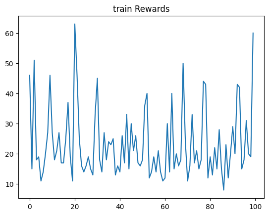
Start testing!
Episode 1 completed in 18 steps
Episode: 1/100, reward: 18.00
Episode 2 completed in 15 steps
Episode: 2/100, reward: 15.00
Episode 3 completed in 22 steps
Episode: 3/100, reward: 22.00
Episode 4 completed in 25 steps
Episode: 4/100, reward: 25.00
Episode 5 completed in 21 steps
Episode: 5/100, reward: 21.00
Episode 6 completed in 33 steps
Episode: 6/100, reward: 33.00
Episode 7 completed in 20 steps
Episode: 7/100, reward: 20.00
Episode 8 completed in 22 steps
Episode: 8/100, reward: 22.00
Episode 9 completed in 30 steps
Episode: 9/100, reward: 30.00
Episode 10 completed in 18 steps
Episode: 10/100, reward: 18.00
Episode 11 completed in 16 steps
Episode: 11/100, reward: 16.00
Episode 12 completed in 20 steps
Episode: 12/100, reward: 20.00
Episode 13 completed in 16 steps
Episode: 13/100, reward: 16.00
Episode 14 completed in 27 steps
Episode: 14/100, reward: 27.00
Episode 15 completed in 13 steps
Episode: 15/100, reward: 13.00
Episode 16 completed in 26 steps
Episode: 16/100, reward: 26.00
Episode 17 completed in 24 steps
Episode: 17/100, reward: 24.00
Episode 18 completed in 15 steps
Episode: 18/100, reward: 15.00
Episode 19 completed in 12 steps
Episode: 19/100, reward: 12.00
Episode 20 completed in 22 steps
Episode: 20/100, reward: 22.00
Episode 21 completed in 52 steps
Episode: 21/100, reward: 52.00
Episode 22 completed in 18 steps
Episode: 22/100, reward: 18.00
Episode 23 completed in 35 steps
Episode: 23/100, reward: 35.00
Episode 24 completed in 47 steps
Episode: 24/100, reward: 47.00
Episode 25 completed in 9 steps
Episode: 25/100, reward: 9.00
Episode 26 completed in 32 steps
Episode: 26/100, reward: 32.00
Episode 27 completed in 12 steps
Episode: 27/100, reward: 12.00
Episode 28 completed in 14 steps
Episode: 28/100, reward: 14.00
Episode 29 completed in 46 steps
Episode: 29/100, reward: 46.00
Episode 30 completed in 55 steps
Episode: 30/100, reward: 55.00
Episode 31 completed in 21 steps
Episode: 31/100, reward: 21.00
Episode 32 completed in 12 steps
Episode: 32/100, reward: 12.00
Episode 33 completed in 9 steps
Episode: 33/100, reward: 9.00
Episode 34 completed in 26 steps
Episode: 34/100, reward: 26.00
Episode 35 completed in 26 steps
Episode: 35/100, reward: 26.00
Episode 36 completed in 20 steps
Episode: 36/100, reward: 20.00
Episode 37 completed in 25 steps
Episode: 37/100, reward: 25.00
Episode 38 completed in 34 steps
Episode: 38/100, reward: 34.00
Episode 39 completed in 13 steps
Episode: 39/100, reward: 13.00
Episode 40 completed in 23 steps
Episode: 40/100, reward: 23.00
Episode 41 completed in 23 steps
Episode: 41/100, reward: 23.00
Episode 42 completed in 30 steps
Episode: 42/100, reward: 30.00
Episode 43 completed in 16 steps
Episode: 43/100, reward: 16.00
Episode 44 completed in 50 steps
Episode: 44/100, reward: 50.00
Episode 45 completed in 13 steps
Episode: 45/100, reward: 13.00
Episode 46 completed in 15 steps
Episode: 46/100, reward: 15.00
Episode 47 completed in 44 steps
Episode: 47/100, reward: 44.00
Episode 48 completed in 11 steps
Episode: 48/100, reward: 11.00
Episode 49 completed in 51 steps
Episode: 49/100, reward: 51.00
Episode 50 completed in 18 steps
Episode: 50/100, reward: 18.00
Episode 51 completed in 11 steps
Episode: 51/100, reward: 11.00
Episode 52 completed in 11 steps
Episode: 52/100, reward: 11.00
Episode 53 completed in 33 steps
Episode: 53/100, reward: 33.00
Episode 54 completed in 19 steps
Episode: 54/100, reward: 19.00
Episode 55 completed in 19 steps
Episode: 55/100, reward: 19.00
Episode 56 completed in 17 steps
Episode: 56/100, reward: 17.00
Episode 57 completed in 10 steps
Episode: 57/100, reward: 10.00
Episode 58 completed in 22 steps
Episode: 58/100, reward: 22.00
Episode 59 completed in 25 steps
Episode: 59/100, reward: 25.00
Episode 60 completed in 28 steps
Episode: 60/100, reward: 28.00
Episode 61 completed in 30 steps
Episode: 61/100, reward: 30.00
Episode 62 completed in 18 steps
Episode: 62/100, reward: 18.00
Episode 63 completed in 54 steps
Episode: 63/100, reward: 54.00
Episode 64 completed in 35 steps
Episode: 64/100, reward: 35.00
Episode 65 completed in 57 steps
Episode: 65/100, reward: 57.00
Episode 66 completed in 27 steps
Episode: 66/100, reward: 27.00
Episode 67 completed in 10 steps
Episode: 67/100, reward: 10.00
Episode 68 completed in 28 steps
Episode: 68/100, reward: 28.00
Episode 69 completed in 31 steps
Episode: 69/100, reward: 31.00
Episode 70 completed in 18 steps
Episode: 70/100, reward: 18.00
Episode 71 completed in 8 steps
Episode: 71/100, reward: 8.00
Episode 72 completed in 16 steps
Episode: 72/100, reward: 16.00
Episode 73 completed in 29 steps
Episode: 73/100, reward: 29.00
Episode 74 completed in 12 steps
Episode: 74/100, reward: 12.00
Episode 75 completed in 38 steps
Episode: 75/100, reward: 38.00
Episode 76 completed in 31 steps
Episode: 76/100, reward: 31.00
Episode 77 completed in 17 steps
Episode: 77/100, reward: 17.00
Episode 78 completed in 29 steps
Episode: 78/100, reward: 29.00
Episode 79 completed in 68 steps
Episode: 79/100, reward: 68.00
Episode 80 completed in 16 steps
Episode: 80/100, reward: 16.00
Episode 81 completed in 24 steps
Episode: 81/100, reward: 24.00
Episode 82 completed in 13 steps
Episode: 82/100, reward: 13.00
Episode 83 completed in 22 steps
Episode: 83/100, reward: 22.00
Episode 84 completed in 11 steps
Episode: 84/100, reward: 11.00
Episode 85 completed in 21 steps
Episode: 85/100, reward: 21.00
Episode 86 completed in 22 steps
Episode: 86/100, reward: 22.00
Episode 87 completed in 16 steps
Episode: 87/100, reward: 16.00
Episode 88 completed in 13 steps
Episode: 88/100, reward: 13.00
Episode 89 completed in 15 steps
Episode: 89/100, reward: 15.00
Episode 90 completed in 14 steps
Episode: 90/100, reward: 14.00
Episode 91 completed in 21 steps
Episode: 91/100, reward: 21.00
Episode 92 completed in 15 steps
Episode: 92/100, reward: 15.00
Episode 93 completed in 24 steps
Episode: 93/100, reward: 24.00
Episode 94 completed in 14 steps
Episode: 94/100, reward: 14.00
Episode 95 completed in 28 steps
Episode: 95/100, reward: 28.00
Episode 96 completed in 56 steps
Episode: 96/100, reward: 56.00
Episode 97 completed in 51 steps
Episode: 97/100, reward: 51.00
Episode 98 completed in 15 steps
Episode: 98/100, reward: 15.00
Episode 99 completed in 22 steps
Episode: 99/100, reward: 22.00
Episode 100 completed in 26 steps
Episode: 100/100, reward: 26.00
Testing complete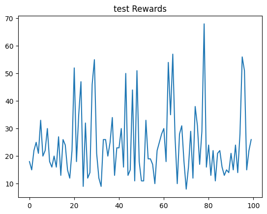
 Actor-Critic Model
The Actor-Critic model is a reinforcement learning framework that combines value-based methods and policy-based methods. Its core idea is to combine the strengths of policy decision making, the actor, and value-function estimation, the critic, to achieve better learning efficiency and policy performance.The actor is responsible for choosing actions based on the current policy。
- This policy is usually stochastic, allowing the algorithm to balance exploration, trying new actions, and exploitation, choosing known good actions. The actor’s policy is implemented in a parameterized form, usually with a neural network. Its parameters are updated by policy gradient methods. Details are as follows:
- Input: The input to the actor network is usually the current state of the environment.
- Output: The output is a probability distribution over possible actions in a discrete action space, or parameters of an action, such as mean and standard deviation, in a continuous action space.
- Loss function: The actor network is usually trained by policy gradient methods, such as REINFORCE or the policy gradient used in Actor-Critic methods.
- Optimization method: Gradient ascent is commonly used to maximize the expected reward.
The critic estimates the value of the selected action
- The value is usually the Q-value of a state-action pair or only the state value V. This evaluation helps the actor judge whether the selected action is good or bad. The critic is usually updated using TD-Learning or other value-function approximation methods, and the value feedback it provides guides the actor’s policy update. Details are as follows:
- Input: The input is usually the current state, or a combination of state and action.
- Output: The output is the value estimate of the current state or state-action pair, namely the Q-value (state-action value function) or V-value (state value function).
- Loss function: The critic’s loss function is usually the squared TD error.
- Optimization method: Gradient descent is the most common method for minimizing the value-estimation error.
In the Actor-Critic model, the learning process involves an interactive process。
- The actor chooses actions.
- The critic evaluates whether these actions are good or bad.
- The following explains each step in detail:
- Step1: Based on the current policy, the actor selects an action.
- Step2: Environment feedback. The environment returns a new state and reward according to the selected action.
- Step3: Learning update. The critic uses the TD error to evaluate the value of the action taken. At the same time, the actor updates its policy based on the critic’s feedback, increasing the probability of choosing more valuable actions in similar situations.
- Step4: Continue iterating until the trajectory ends.
Advantages and disadvantages of the Actor-Critic algorithm
- Advantages:
1. Combining stability and efficiency: The Actor-Critic model combines the strengths of policy-based methods, such as REINFORCE, and value-based methods, such as Q-learning or DQN. It is more stable and efficient than using a pure policy gradient method or a pure value-function method alone.
2. Suitable for continuous action spaces: Unlike value-only methods such as DQN, the Actor-Critic model can handle continuous action spaces. This makes it more effective for problems such as robot control. This advantage comes from policy-based reinforcement learning.
3. Reduced variance and improved learning efficiency: Introducing the critic helps reduce the variance of policy estimation and improves learning efficiency. This advantage comes from value-based reinforcement learning.
4. Online and offline learning: It can be used for online learning, learning from each step, and offline learning, learning from a complete episode. This provides flexible learning modes.
- Disadvantages:
- Complexity and computational cost: Two models, the actor and the critic, must be trained at the same time. This can make the model more complex and computationally expensive.
- Stability issues: Although it is more stable than pure policy gradient methods, Actor-Critic is still less stable than traditional value-based methods such as DQN.
- Hyperparameter tuning difficulty: More hyperparameters must be tuned, such as learning rates for two networks and the discount factor. Tuning may be harder than for a single-model method.
- Risk of overestimation: The critic may overestimate the value function, especially when using function approximators such as neural networks. This can make learning unstable.
Example Code: Actor-Critic Model
class ActorCriticNetwork(nn.Module):
    def __init__(self, n_states, n_actions):
        super(ActorCriticNetwork, self).__init__()
        self.fc1 = nn.Linear(n_states, 256)
        self.fc2 = nn.Linear(256, 128)
        self.actor = nn.Linear(128, n_actions)
        self.critic = nn.Linear(128, 1)

    def forward(self, x):
        x = F.relu(self.fc1(x))
        x = F.relu(self.fc2(x))
        policy_dist = F.softmax(self.actor(x), dim=-1)
        value = self.critic(x)
        return policy_dist, value
class ActorCritic:
    def __init__(self, model, memory, cfg):
        self.n_actions = cfg['n_actions']
        self.device = torch.device(cfg['device'])
        self.gamma = cfg['gamma']
        self.model = model.to(self.device)
        self.optimizer = optim.Adam(self.model.parameters(), lr=cfg['lr'])
        self.memory = memory

    # Sample an action method
    def sample_action(self, state):
        state = torch.tensor(state, device=self.device, dtype=torch.float32).unsqueeze(dim=0)  # Convert the state to a tensor
        policy_dist, _ = self.model(state)  # Get the policy distribution
        policy_dist = policy_dist.cpu().detach().numpy().flatten()  # Convert the policy distribution to a NumPy array and flatten it
        action = np.random.choice(self.n_actions, p=policy_dist)  # Sample an action from the policy distribution
        return action

    # Update the model
    def update(self):
        if len(self.memory) < self.memory.capacity:  # If the buffer does not contain enough experiences
            return
        # Sample a batch of experiences from the buffer
        state_batch, action_batch, reward_batch, next_state_batch, done_batch = self.memory.sample(self.memory.capacity)
        state_batch = torch.tensor(np.array(state_batch), device=self.device, dtype=torch.float32)  # Convert the state to a tensor
        action_batch = torch.tensor(action_batch, device=self.device)  # Convert actions to tensors
        reward_batch = torch.tensor(reward_batch, device=self.device, dtype=torch.float32)  # Convert rewards to tensors
        next_state_batch = torch.tensor(np.array(next_state_batch), device=self.device, dtype=torch.float32)  # Convert next states to tensors
        done_batch = torch.tensor(done_batch, device=self.device, dtype=torch.float32)  # Convert done flags to tensors

        # Get the value of the next state
        _, next_value = self.model(next_state_batch)
        # Compute target values
        target_values = reward_batch + self.gamma * next_value.squeeze() * (1 - done_batch)

        # Get the current-state policy distribution and value
        policy_dist, values = self.model(state_batch)
        values = values.squeeze()  # Remove extra dimensions

        # Compute advantages
        advantages = target_values - values

        # Compute the log probability of the policy
        log_probs = torch.log(policy_dist.gather(1, action_batch.unsqueeze(1)))
        actor_loss = -torch.sum(log_probs.squeeze() * advantages.detach())  # policy loss
        critic_loss = F.mse_loss(values, target_values.detach())  # value loss

        loss = actor_loss + critic_loss  # total loss

        self.optimizer.zero_grad()
        loss.backward()
        self.optimizer.step()
def env_agent_config(cfg):
    env = gym.make(cfg['env_name'])
    n_states = env.observation_space.shape[0]
    n_actions = env.action_space.n
    memory = ReplayBuffer(cfg['memory_capacity'])
    agent = ActorCritic(ActorCriticNetwork(n_states, n_actions), memory, cfg)
    return env, agent

def train(cfg, env, agent):
    print("Start training!")
    rewards = []
    steps = []
    for i_ep in range(cfg['train_eps']):
        ep_reward = 0
        ep_step = 0
        state, _ = env.reset()
        done = False
        while not done:
            ep_step += 1
            action = agent.sample_action(state)
            next_state, reward, done, truncated, _ = env.step(action)
            done = done or truncated
            agent.memory.push((state, action, reward, next_state, done))
            state = next_state
            ep_reward += reward
            if done:
                break
        agent.update()
        steps.append(ep_step)
        rewards.append(ep_reward)
        if (i_ep + 1) % 10 == 0:
            print(f"episode:{i_ep + 1}/{cfg['train_eps']},reward:{ep_reward:.2f}")
    print("Training complete!")
    env.close()
    return {'rewards': rewards}

def test(cfg, env, agent):
    print("Start testing!")
    rewards = []
    steps = []
    for i_ep in range(cfg['test_eps']):
        ep_reward = 0
        ep_step = 0
        state, _ = env.reset()
        done = False
        while not done and ep_step < cfg['ep_max_steps']:
            ep_step += 1
            action = agent.sample_action(state)
            next_state, reward, done, truncated, _ = env.step(action)
            done = done or truncated
            state = next_state
            ep_reward += reward
            if done:
                print(f"episode {i_ep + 1} completed in {ep_step} steps")
        steps.append(ep_step)
        rewards.append(ep_reward)
        print(f"episode:{i_ep + 1}/{cfg['test_eps']},reward:{ep_reward:.2f}")
    print("Testing complete")
    env.close()
    return {'rewards': rewards}

def get_args():
    return {
        'env_name': 'CartPole-v1',
        'n_actions': 2,
        'device': 'cpu',
        'gamma': 0.99,  # Adjust the discount factor
        'lr': 0.0005,  # Adjust the learning rate
        'memory_capacity': 10000,
        'train_eps': 100,  # Increase the number of training episodes
        'test_eps': 100,
        'ep_max_steps': 200,
        'seed': 42
    }

def plot_rewards(rewards, cfg, tag="train"):
    import matplotlib.pyplot as plt
    plt.plot(rewards)
    plt.title(f'{tag} Rewards')
    plt.show()

cfg = get_args()
env, agent = env_agent_config(cfg)
res_dic = train(cfg, env, agent)
plot_rewards(res_dic['rewards'], cfg, tag="train")
res_dic = test(cfg, env, agent)
plot_rewards(res_dic['rewards'], cfg, tag="test")
Start training!
Episode: 10/100, reward: 19.00
Episode: 20/100, reward: 10.00
Episode: 30/100, reward: 11.00
Episode: 40/100, reward: 11.00
Episode: 50/100, reward: 36.00
Episode: 60/100, reward: 34.00
Episode: 70/100, reward: 28.00
Episode: 80/100, reward: 81.00
Episode: 90/100, reward: 25.00
Episode: 100/100, reward: 26.00
Training complete!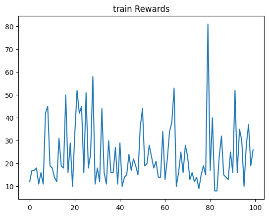
Start testing!
Episode 1 completed in 19 steps
Episode: 1/100, reward: 19.00
Episode 2 completed in 13 steps
Episode: 2/100, reward: 13.00
Episode 3 completed in 16 steps
Episode: 3/100, reward: 16.00
Episode 4 completed in 11 steps
Episode: 4/100, reward: 11.00
Episode 5 completed in 10 steps
Episode: 5/100, reward: 10.00
Episode 6 completed in 19 steps
Episode: 6/100, reward: 19.00
Episode 7 completed in 10 steps
Episode: 7/100, reward: 10.00
Episode 8 completed in 43 steps
Episode: 8/100, reward: 43.00
Episode 9 completed in 18 steps
Episode: 9/100, reward: 18.00
Episode 10 completed in 17 steps
Episode: 10/100, reward: 17.00
Episode 11 completed in 11 steps
Episode: 11/100, reward: 11.00
Episode 12 completed in 15 steps
Episode: 12/100, reward: 15.00
Episode 13 completed in 22 steps
Episode: 13/100, reward: 22.00
Episode 14 completed in 21 steps
Episode: 14/100, reward: 21.00
Episode 15 completed in 13 steps
Episode: 15/100, reward: 13.00
Episode 16 completed in 9 steps
Episode: 16/100, reward: 9.00
Episode 17 completed in 8 steps
Episode: 17/100, reward: 8.00
Episode 18 completed in 17 steps
Episode: 18/100, reward: 17.00
Episode 19 completed in 44 steps
Episode: 19/100, reward: 44.00
Episode 20 completed in 12 steps
Episode: 20/100, reward: 12.00
Episode 21 completed in 30 steps
Episode: 21/100, reward: 30.00
Episode 22 completed in 19 steps
Episode: 22/100, reward: 19.00
Episode 23 completed in 21 steps
Episode: 23/100, reward: 21.00
Episode 24 completed in 28 steps
Episode: 24/100, reward: 28.00
Episode 25 completed in 14 steps
Episode: 25/100, reward: 14.00
Episode 26 completed in 9 steps
Episode: 26/100, reward: 9.00
Episode 27 completed in 25 steps
Episode: 27/100, reward: 25.00
Episode 28 completed in 26 steps
Episode: 28/100, reward: 26.00
Episode 29 completed in 20 steps
Episode: 29/100, reward: 20.00
Episode 30 completed in 12 steps
Episode: 30/100, reward: 12.00
Episode 31 completed in 22 steps
Episode: 31/100, reward: 22.00
Episode 32 completed in 22 steps
Episode: 32/100, reward: 22.00
Episode 33 completed in 26 steps
Episode: 33/100, reward: 26.00
Episode 34 completed in 21 steps
Episode: 34/100, reward: 21.00
Episode 35 completed in 17 steps
Episode: 35/100, reward: 17.00
Episode 36 completed in 22 steps
Episode: 36/100, reward: 22.00
Episode 37 completed in 12 steps
Episode: 37/100, reward: 12.00
Episode 38 completed in 25 steps
Episode: 38/100, reward: 25.00
Episode 39 completed in 10 steps
Episode: 39/100, reward: 10.00
Episode 40 completed in 15 steps
Episode: 40/100, reward: 15.00
Episode 41 completed in 10 steps
Episode: 41/100, reward: 10.00
Episode 42 completed in 9 steps
Episode: 42/100, reward: 9.00
Episode 43 completed in 22 steps
Episode: 43/100, reward: 22.00
Episode 44 completed in 15 steps
Episode: 44/100, reward: 15.00
Episode 45 completed in 15 steps
Episode: 45/100, reward: 15.00
Episode 46 completed in 12 steps
Episode: 46/100, reward: 12.00
Episode 47 completed in 29 steps
Episode: 47/100, reward: 29.00
Episode 48 completed in 14 steps
Episode: 48/100, reward: 14.00
Episode 49 completed in 16 steps
Episode: 49/100, reward: 16.00
Episode 50 completed in 18 steps
Episode: 50/100, reward: 18.00
Episode 51 completed in 18 steps
Episode: 51/100, reward: 18.00
Episode 52 completed in 18 steps
Episode: 52/100, reward: 18.00
Episode 53 completed in 12 steps
Episode: 53/100, reward: 12.00
Episode 54 completed in 15 steps
Episode: 54/100, reward: 15.00
Episode 55 completed in 19 steps
Episode: 55/100, reward: 19.00
Episode 56 completed in 36 steps
Episode: 56/100, reward: 36.00
Episode 57 completed in 44 steps
Episode: 57/100, reward: 44.00
Episode 58 completed in 21 steps
Episode: 58/100, reward: 21.00
Episode 59 completed in 22 steps
Episode: 59/100, reward: 22.00
Episode 60 completed in 22 steps
Episode: 60/100, reward: 22.00
Episode 61 completed in 23 steps
Episode: 61/100, reward: 23.00
Episode 62 completed in 53 steps
Episode: 62/100, reward: 53.00
Episode 63 completed in 10 steps
Episode: 63/100, reward: 10.00
Episode 64 completed in 26 steps
Episode: 64/100, reward: 26.00
Episode 65 completed in 20 steps
Episode: 65/100, reward: 20.00
Episode 66 completed in 26 steps
Episode: 66/100, reward: 26.00
Episode 67 completed in 13 steps
Episode: 67/100, reward: 13.00
Episode 68 completed in 11 steps
Episode: 68/100, reward: 11.00
Episode 69 completed in 19 steps
Episode: 69/100, reward: 19.00
Episode 70 completed in 20 steps
Episode: 70/100, reward: 20.00
Episode 71 completed in 11 steps
Episode: 71/100, reward: 11.00
Episode 72 completed in 31 steps
Episode: 72/100, reward: 31.00
Episode 73 completed in 25 steps
Episode: 73/100, reward: 25.00
Episode 74 completed in 34 steps
Episode: 74/100, reward: 34.00
Episode 75 completed in 13 steps
Episode: 75/100, reward: 13.00
Episode 76 completed in 21 steps
Episode: 76/100, reward: 21.00
Episode 77 completed in 9 steps
Episode: 77/100, reward: 9.00
Episode 78 completed in 16 steps
Episode: 78/100, reward: 16.00
Episode 79 completed in 17 steps
Episode: 79/100, reward: 17.00
Episode 80 completed in 42 steps
Episode: 80/100, reward: 42.00
Episode 81 completed in 16 steps
Episode: 81/100, reward: 16.00
Episode 82 completed in 19 steps
Episode: 82/100, reward: 19.00
Episode 83 completed in 18 steps
Episode: 83/100, reward: 18.00
Episode 84 completed in 23 steps
Episode: 84/100, reward: 23.00
Episode 85 completed in 22 steps
Episode: 85/100, reward: 22.00
Episode 86 completed in 45 steps
Episode: 86/100, reward: 45.00
Episode 87 completed in 26 steps
Episode: 87/100, reward: 26.00
Episode 88 completed in 87 steps
Episode: 88/100, reward: 87.00
Episode 89 completed in 14 steps
Episode: 89/100, reward: 14.00
Episode 90 completed in 11 steps
Episode: 90/100, reward: 11.00
Episode 91 completed in 15 steps
Episode: 91/100, reward: 15.00
Episode 92 completed in 12 steps
Episode: 92/100, reward: 12.00
Episode 93 completed in 19 steps
Episode: 93/100, reward: 19.00
Episode 94 completed in 23 steps
Episode: 94/100, reward: 23.00
Episode 95 completed in 19 steps
Episode: 95/100, reward: 19.00
Episode 96 completed in 14 steps
Episode: 96/100, reward: 14.00
Episode 97 completed in 18 steps
Episode: 97/100, reward: 18.00
Episode 98 completed in 28 steps
Episode: 98/100, reward: 28.00
Episode 99 completed in 14 steps
Episode: 99/100, reward: 14.00
Episode 100 completed in 24 steps
Episode: 100/100, reward: 24.00
Testing complete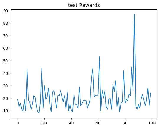
Generative Adversarial Networks vs. Actor-Critic Algorithms
First, let us briefly review these two models.Generative Adversarial Networks (GANs)
- Basic concept: GANs consist of two parts, a generator and a discriminator. The generator aims to create realistic data, such as images, while the discriminator aims to distinguish real data from fake data produced by the generator.
- Training nature: In GANs, the generator and discriminator have an adversarial relationship. The generator tries to fool the discriminator, while the discriminator tries not to be fooled. This adversarial process improves both models, and eventually the generator can produce highly realistic data.
- Learning mechanism: The learning process in GANs is a dynamic equilibrium game. The generator continually improves the data it generates to avoid detection by the discriminator, while the discriminator continually improves its ability to distinguish real from fake data.
Actor-Critic Model
- Basic concept: The Actor-Critic model consists of two parts, the actor and the critic. The actor selects actions, and the critic evaluates these actions and provides feedback.
- Training nature: Unlike GANs, the actor and critic in an Actor-Critic model have a cooperative relationship. The critic’s feedback helps the actor improve its policy and optimize action selection.
- Learning mechanism: In the Actor-Critic model, the actor’s action selection is guided by the value estimates provided by the critic. The critic adjusts its own value estimates based on the actor’s performance. This mechanism helps optimize both policy selection and value judgment.
Q1: Why is the training nature adversarial in one case and cooperative in the other?
Q2: Which is better: adversarial improvement or cooperative win-win learning?
 Credits
- Icons made by Becris from www.flaticon.com
- Icons from Icons8.com – https://icons8.com
- Dive Into Deep Learning – Recurrent Neural Networks
- DS-GA 1008 – NYU CENTER FOR DATA SCIENCE – Deep Sequence Modeling
- Text classification with the torchtext library
- Tricks For Training Transformers – Borealis AI – P. Xu, S. Prince
- Tal Daniel