Deep Learning

---

created by Deepfinder

Agenda

---

1. Teaching by example: Supervised Learning
2. Learning from patterns: Unsupervised Learning
3. Learning without labels: Self-supervised Learning
4. Learning from a few labels: Semi-supervised Learning
5. Learning by comparison: Contrastive Learning
6. Generalizing from one task to another: Transfer Learning
7. Learning through opposition: Adversarial Learning
8. Working together: Ensemble Learning
9. Different paths to one goal: Federated Learning
10. Learning through trial and error: Reinforcement Learning
11. Learning by asking: Active Learning
12. Learning to learn: Meta-Learning

Motivation for Active Learning

---

Active learning is a machine learning paradigm. It aims to select the most valuable samples for labeling, so that we can reduce labeling cost while improving model performance.

The core idea of active learning is simple: let the model actively choose the samples that are most helpful for its own learning, instead of selecting samples at random. In this way, active learning can train a better model with fewer labeled samples.

The core principle of a support vector machine (SVM) is to define the decision boundary using a small number of support vectors, rather than relying on the whole dataset. These support vectors are the points closest to the decision boundary, and they determine the final shape of the classifier. In active learning, this property matches the main idea of active learning: both methods try to identify the most important information from a large amount of data.

---

Basic components of Active Learning

• Unlabeled Data Pool: a large set of unlabeled data. This is the basis of active learning.

• Labeled Data Set: it may be empty at the beginning, and then gradually grows during learning.

• Learner: the model trained from the labeled data.

• Oracle: the process that provides the true labels. It is usually a human annotator.

Common methods in active learning

• Uncertainty Sampling: select the samples for which the model is most uncertain.

• Common criteria:

  ○ Least Confidence: select the samples for which the model is least confident.

  ○ Minimum Margin: select the samples where the model hesitates between the two most likely classes.

  ○ Entropy: select the samples with the highest prediction entropy.

• Query-by-Committee, QBC: use the disagreement between several models, called a committee, to select samples.

• Common criteria:

  ○ Vote Entropy: compute entropy from the voting results of committee members.

  ○ Consensus Entropy: compute entropy from the probability estimates of committee members.

  ○ KL Divergence (Kullback-Leibler Divergence): measure the disagreement between committee members and the overall consensus.

• Expected Model Change, EMC:

  ○ Select the samples that can change the model the most.

  ○ Approximate model change by computing the expected length of the gradient.

• Expected Error Reduction, EER:

  ○ Select the samples that can reduce the model error on future data the most.

  ○ This requires retraining the model, so the computational cost is high.

• Density Weighting:

  ○ When selecting samples, consider not only model uncertainty, but also the density of samples in the data distribution.

  ○ This avoids selecting samples from sparse regions or outliers.

%matplotlib inline
import numpy as np
import matplotlib.pyplot as plt
from scipy.stats import multivariate_normal, ortho_group
from sklearn.linear_model import LogisticRegression
import seaborn as sns
from typing import Callable, Sequence, Tuple, Optional
from random import choice

# Set the Seaborn style
sns.set_style("white")
colors = sns.color_palette(n_colors=10)

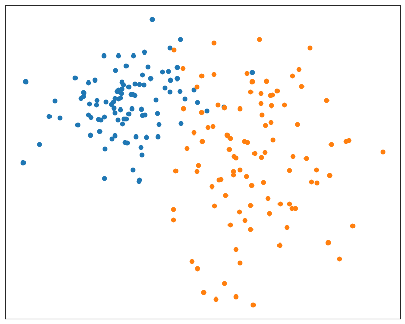
Sample two-dimensional data from two Gaussian distributions. Adjust the random seed to obtain Gaussian distributions with different shapes.

# Define a helper function
def sample_covar(dim: int = 2, scale_min: float = 0.3, scale_max: float = 5) -> np.ndarray:
    """Construct random covariance matrix by sampling a rotation and scale matrix."""
    R = ortho_group.rvs(dim) * (np.random.rand(dim, dim) * (scale_max - scale_min) + scale_min)
    return R.dot(R.T)

# Generate example data
N_1, N_2 = 100, 100  # number of samples in each point cloud
mu_1 = [-5, 2]  # centroid of the first point cloud
mu_2 = [5, -2]  # centroid of the second point cloud

np.random.seed(27)

X = np.concatenate([
    multivariate_normal(mu_1, sample_covar()).rvs(N_1),
    multivariate_normal(mu_2, sample_covar()).rvs(N_2),
])
y = np.concatenate([np.zeros(N_1, int), np.ones(N_2, int)])

# Show a scatter plot of the data
plt.figure(figsize=(10, 8))
plt.scatter(X[y == 0, 0], X[y == 0, 1], color=colors[0])
plt.scatter(X[y == 1, 0], X[y == 1, 1], color=colors[1])
plt.xticks(()), plt.yticks(())
plt.show()

Helper functions for plotting data and classifiers (not important)

# Define helper functions
def meshgrid_from_bounds(lower_left: Sequence[float], upper_right: Sequence[float], *,
                         resolution: float = 0.02) -> Tuple[np.ndarray, np.ndarray]:
    """Return a meshgrid that covers the range from lower_left to upper_right."""
    return np.meshgrid(np.arange(lower_left[0], upper_right[0], resolution),
                       np.arange(lower_left[1], upper_right[1], resolution))

def plot_decision_boundary(clf, lower_left: Sequence[float], upper_right: Sequence[float], *,
                           resolution: float = 0.02, boundary_color: Tuple[float] = (0.2, 0.2, 0.2)):
    """Plot decision boundary of a given classifier in the given range."""
    xx, yy = meshgrid_from_bounds(lower_left, upper_right, resolution=resolution)
    Z = clf.predict_proba(np.c_[xx.ravel(), yy.ravel()])[:, 0].reshape(xx.shape)
    plt.contour(xx, yy, Z, levels=[0.5], colors=[boundary_color])

def lighten(color: Tuple[float], *, amount: float = 0.6):
    """Blend color with white by the given amount."""
    return tuple(np.array(color) * (1 - amount) + np.array([1, 1, 1]) * amount)

def plot_data(X: np.ndarray, y: np.ndarray, train_idx: Sequence[int], *,
              colors: Sequence[Tuple[float]] = sns.color_palette(n_colors=2)):
    """Scatter plot of the training and unlabeled data."""
    # Show all data
    plt.scatter(X[y == 0, 0], X[y == 0, 1], color=lighten(colors[0]), s=6)
    plt.scatter(X[y == 1, 0], X[y == 1, 1], color=lighten(colors[1]), s=6)

    # Show training data
    X_tr = X[train_idx]
    y_tr = y[train_idx]
    plt.scatter(X_tr[y_tr == 0, 0], X_tr[y_tr == 0, 1], color=colors[0])
    plt.scatter(X_tr[y_tr == 1, 0], X_tr[y_tr == 1, 1], color=colors[1])
    plt.xticks(()), plt.yticks(())

def plot_data_and_classifier(X: np.ndarray, y: np.ndarray, train_idx: Sequence[int], clf, *,
                             previous_clf=None, colors: Sequence[Tuple[float]] = sns.color_palette(n_colors=2)):
    """Scatter plot of the training and unlabeled data and the decision boundary of the classifier."""
    if previous_clf is not None:
        plot_decision_boundary(previous_clf, lower_left=X.min(axis=0) - 1, upper_right=X.max(axis=0) + 1, boundary_color=(0.7, 0.7, 0.7))

    plot_decision_boundary(clf, lower_left=X.min(axis=0) - 1, upper_right=X.max(axis=0) + 1)
    plot_data(X, y, train_idx, colors=colors)

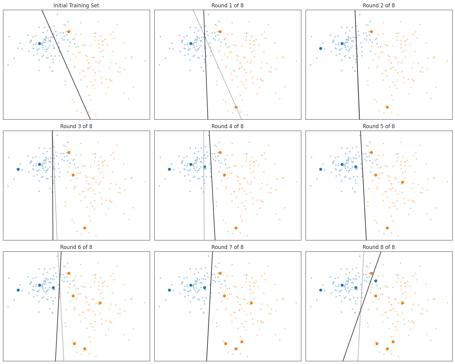
Non-active Learning

# Initialize the random seed
np.random.seed(42)  # Choose a fixed random seed

# Randomly select one sample from each class as the initial training set
starting_samples = [choice(range(N_1)), N_1 + choice(range(N_2))]
train_idx = starting_samples[:]
clf = LogisticRegression().fit(X[train_idx], y[train_idx])

# Plot the initial training set and classifier
plt.figure(figsize=(15, 12))
plt.subplot(3, 3, 1)
plt.title('Initial Training Set')
plot_data_and_classifier(X, y, train_idx, clf)

# Run 8 rounds of random sampling
for round_num in range(8):  
    new_sample = choice([i for i in range(N_1 + N_2) if i not in train_idx])
    train_idx.append(new_sample)
    previous_clf = clf
    clf = LogisticRegression().fit(X[train_idx], y[train_idx])

    ax = plt.subplot(3, 3, round_num + 2)
    plt.title(f'Round {round_num + 1} of 8')
    plot_data_and_classifier(X, y, train_idx, clf, previous_clf=previous_clf)

plt.tight_layout()
plt.show()

Uncertainty Sampling

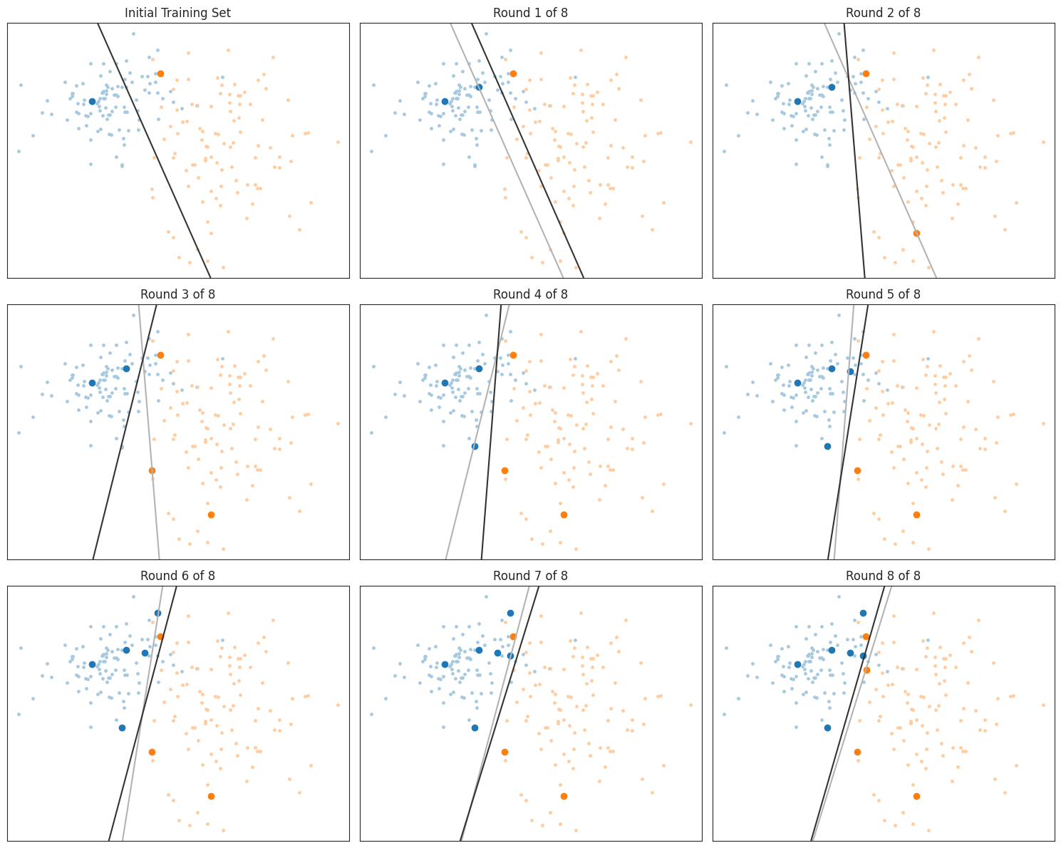
The simplest idea is this: the more uncertain the model is about a sample, the more valuable it is to label that sample. This method is called uncertainty sampling. It applies to any model that can estimate its own prediction uncertainty. For example, some models can output the probability of each class, written as $\hat{P}(y \mid x)$ . We can measure uncertainty using the probability of the most likely class:

$$
u(x)=1-\max _y \hat{P}(y \mid x)
$$

This criterion is called the least confidence score. It selects the samples where the model has the least confidence, meaning that the probabilities of all classes are similar.

Minimum Margin Score

Besides the least confidence score, another case is also worth attention. Sometimes the model can rule out some classes, but the two remaining most likely classes have almost equal probabilities. In this case, we can use the minimum margin score:

$$
u(x)=\hat{P}\left(y_2* \mid x\right)-\hat{P}\left(y_1* \mid x\right)
$$

Here, $y_1*$ and $y_2*$ are the most likely and second most likely classes according to the model. This criterion selects the samples where the model hesitates between two classes. These samples are usually near the decision boundary between the two classes.

Entropy Score

The third criterion comes from information theory and is called the entropy score. Entropy can be understood as the degree of disorder. Here it represents the model uncertainty about the class of a sample. The formula is:

$$
u(x)=\mathbb{E}[-\log \hat{P}(y \mid x)]
$$

In simple terms, the entropy score measures how much information the model would gain after knowing the label of a sample. If the model is very certain about the class, the entropy score is low. If the model is unsure, the entropy score is high. This criterion is similar to the minimum margin score, but it considers all classes, not only the two most likely classes.

In plain language, the core idea of uncertainty sampling is: let the model decide which samples are most worth labeling. By selecting the samples where the model is most uncertain, we can train a better model with less labeled data.

from scipy.stats import entropy
import numpy as np
import matplotlib.pyplot as plt
from sklearn.linear_model import LogisticRegression
from typing import Callable, Sequence

# Define uncertainty sampling criteria
def least_confidence(posterior: np.ndarray) -> np.ndarray:
    """Least confidence criterion, u(x) = 1 - max P(y | x)."""
    return 1 - posterior.max(axis=1)

def minimum_margin(posterior: np.ndarray) -> np.ndarray:
    """Minimum margin criterion, u(x) = P(y_2* | x) - P(y_1* | x), where y_1* and y_2* are the two most probable classes."""
    most_probable = posterior.max(axis=1)
    mask_most_probable = (posterior == most_probable.reshape(-1, 1))
    second_most_probable = (posterior - mask_most_probable).max(axis=1)
    return second_most_probable - most_probable

def entropy_criterion(posterior: np.ndarray) -> np.ndarray:
    """Entropy criterion, u(x) = -E[log P(y | x)]."""
    return entropy(posterior, axis=1)

def uncertainty_sampling(clf, X: np.ndarray, train_idx: Sequence[int], criterion: Callable[[np.ndarray], np.ndarray]) -> int:
    """Get the index of an unknown sample where the classifier is most uncertain about the label."""
    unknown_indices = np.array([i for i in range(X.shape[0]) if i not in train_idx])
    posterior = clf.predict_proba(X[unknown_indices])
    utility = criterion(posterior)
    return unknown_indices[np.argmax(utility)]

# Initialize the training set and classifier
train_idx = starting_samples[:]
clf = LogisticRegression().fit(X[train_idx], y[train_idx])

# Plot the initial training set and classifier
plt.figure(figsize=(15, 12))
plt.subplot(3, 3, 1)
plt.title('Initial Training Set')
plot_data_and_classifier(X, y, train_idx, clf)

# Run 8 rounds of uncertainty sampling
for round_num in range(8):  # Avoid conflict with the built-in function round
    new_sample = uncertainty_sampling(clf, X, train_idx, criterion=entropy_criterion)
    train_idx.append(new_sample)

    plt.subplot(3, 3, round_num + 2)
    plt.title(f'Round {round_num + 1} of 8')
    previous_clf = clf
    clf = LogisticRegression().fit(X[train_idx], y[train_idx])
    plot_data_and_classifier(X, y, train_idx, clf, previous_clf=previous_clf)

plt.tight_layout()
plt.show()

Query-by-Committee

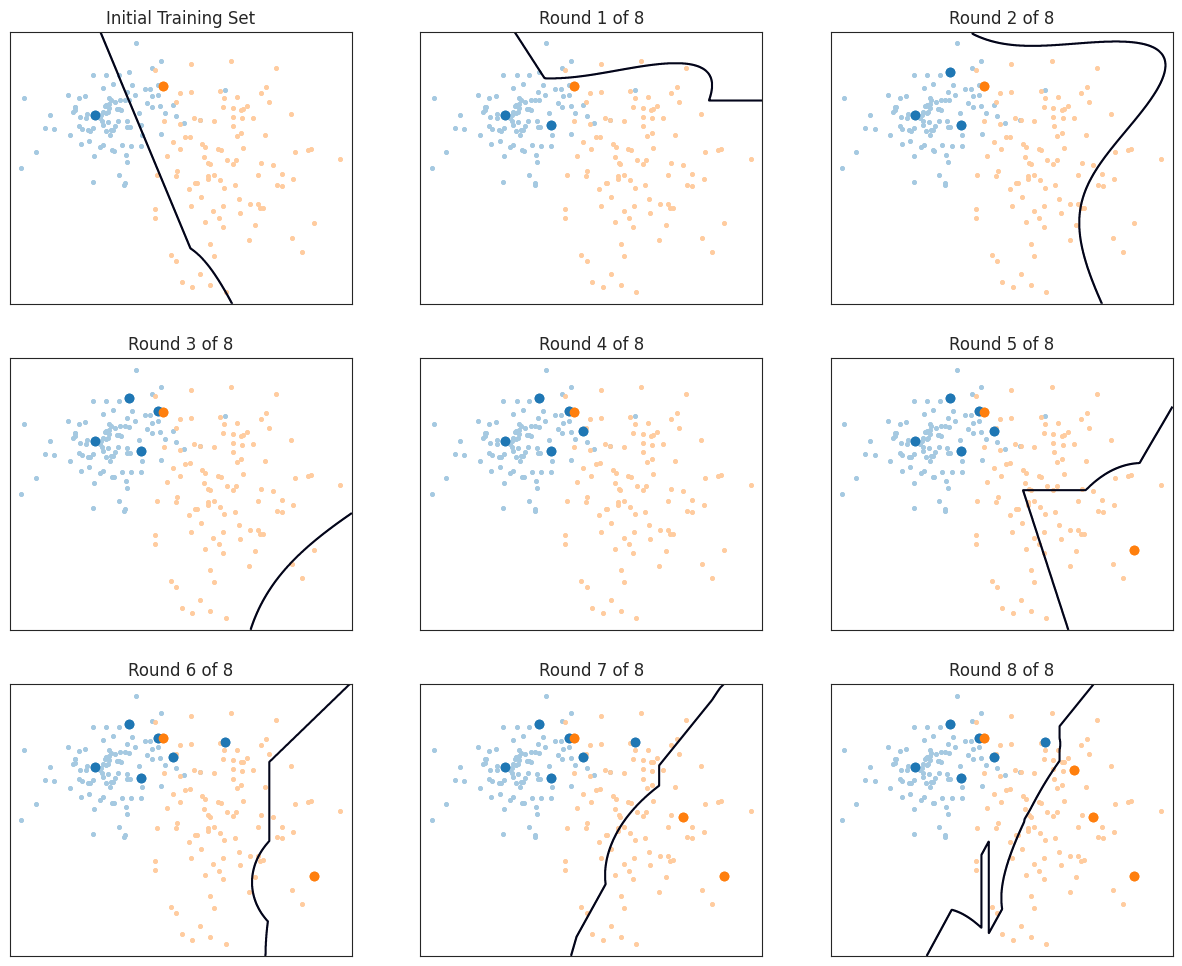
Query-by-Committee (QBC) is inspired by ensemble learning methods. It does not use only one classifier. Instead, it considers the decisions of a committee of multiple classifiers, written as $C=h_1, \ldots, h_C$ . Each classifier has the same target classes, but the underlying model or the view of the data is different. Random forest is a typical example: each classifier is a decision tree, but each tree is trained on a different subset of features.

How do we decide whether an unlabeled sample is valuable?

The idea is simple. If committee members agree on the class of a sample, then we do not need to label that sample again. If committee members disagree, then we should ask the oracle, such as a human annotator, for the label of this sample. In other words, the degree of disagreement in the committee can represent the value of the sample.

How do we measure disagreement?

If the committee has many members, we can estimate the class probability using the number of votes $V(y)$ for each class $y$:

$$
\hat{P}(y \mid x) \approx \frac{V(y)}{C}
$$

However, the number of classifiers $C$ in a committee is usually not large enough to produce reliable probability estimates. In this case, we can use the entropy mentioned earlier to measure disagreement. This method is called Vote Entropy:

$$
u(x)=-\sum_y \frac{V(y)}{C} \log \frac{V(y)}{C}
$$

Here, $V(y)=\left|\left\lbrace h_i \mid h_i(x)=y \right\rbrace \right|$ is the number of classifiers that vote for class $y$.

import numpy as np
from sklearn.ensemble import VotingClassifier
from sklearn.svm import LinearSVC, SVC
from sklearn.tree import DecisionTreeClassifier
from sklearn.linear_model import PassiveAggressiveClassifier
from sklearn.naive_bayes import GaussianNB
from sklearn.neighbors import KNeighborsClassifier
from scipy.stats import entropy
from matplotlib.pyplot import figure, subplot, title, contour, show
from numpy import array, argmax, meshgrid, apply_along_axis, bincount, ravel, c_

# Return the voting results of the ensemble classifier for each sample in X
def get_ensemble_votes(ensemble, X: np.ndarray, n_classes) -> np.ndarray: 
    predictions = ensemble._predict(X)
    return np.apply_along_axis(np.bincount, axis=1, arr=predictions, minlength=n_classes) # Count votes for each sample prediction and make sure every class is counted.

# Compute the vote entropy of unlabeled samples and return the index of the sample with the largest entropy.
def vote_entropy(ensemble: VotingClassifier, X: np.ndarray, train_idx: Sequence[int], n_classes: int) -> int:
    unknown_indices = array([i for i in range(X.shape[0]) if i not in train_idx])
    votes = get_ensemble_votes(ensemble, X[unknown_indices], n_classes=n_classes)
    utility = entropy(votes / len(ensemble.estimators), axis=1)
    return unknown_indices[argmax(utility)]

def plot_ensemble_voting_decision_boundary(ensemble, X, y, train_idx):
    xx, yy = meshgrid_from_bounds(X.min(0) - 1, X.max(0) + 1)

    try:
        proba = ensemble.predict_proba(np.c_[xx.ravel(), yy.ravel()])
    except AttributeError:
        votes = get_ensemble_votes(ensemble, np.c_[xx.ravel(), yy.ravel()], n_classes=len(np.unique(y)))
        proba = (votes / len(ensemble.estimators))

    contour(xx, yy, proba[:, 0].reshape(xx.shape), levels=[0.5])
    plot_data(X, y, train_idx)

train_idx = starting_samples[:]
# Hard voting
ensemble = VotingClassifier([
    ('linear svm', LinearSVC(dual=False)),
    ('rbf svm', SVC()),
    ('poly svm', SVC(kernel='poly')),
    ('decision tree', DecisionTreeClassifier()),
    ('passive agressive', PassiveAggressiveClassifier()),
    ('naive bayes', GaussianNB()),
    ('knn', KNeighborsClassifier(n_neighbors=2))
], voting='hard').fit(X[train_idx], y[train_idx])

figure(figsize=(15, 12))
subplot(3, 3, 1)
title(f'Initial Training Set')
plot_ensemble_voting_decision_boundary(ensemble, X, y, train_idx)
plot_data(X, y, train_idx)

for round in range(8):
    new_sample = vote_entropy(ensemble, X, train_idx, n_classes=2)
    train_idx.append(new_sample)

    subplot(3, 3, round+2)
    title(f'Round {round + 1} of 8')
    ensemble = ensemble.fit(X[train_idx], y[train_idx])
    plot_ensemble_voting_decision_boundary(ensemble, X, y, train_idx)
    plot_data(X, y, train_idx)

show()

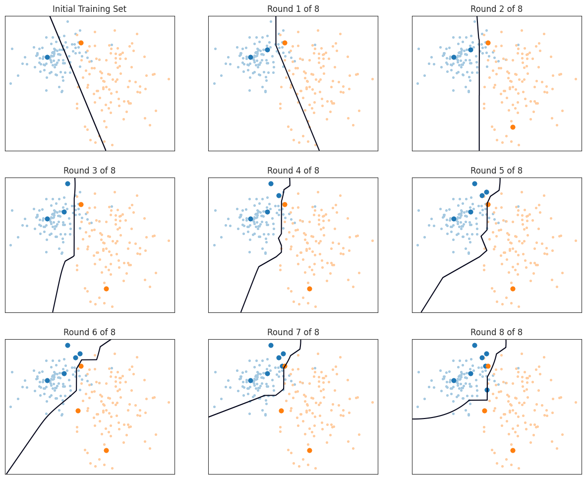
Consensus Entropy

Query the label of the sample that maximizes $u(\mathbf x) = -\sum_y\overline P(y|\mathbf x)\log \overline P(y|\mathbf x)$.

$\overline P(y|\mathbf x) = \frac{1}{C} \sum_{h_i \in \mathcal C} \hat P_i(y|\mathbf x)$ is the consensus probability for class $y$, and $\hat P_i(y|\mathbf x)$ is the posterior class probability estimated by classifier $h_i$ in the ensemble $\mathcal C$.

def consensus_entropy(ensemble: VotingClassifier, X: np.ndarray, train_idx: Sequence[int]) -> int:
  unknown_indices = array([i for i in range(X.shape[0]) if i not in train_idx])
  probas = ensemble.predict_proba(X[unknown_indices])
  utility = entropy(probas, axis=1)
  return unknown_indices[argmax(utility)]

train_idx = starting_samples[:]
ensemble = VotingClassifier([
  ('logistic regression', LogisticRegression()),
  ('decision tree', DecisionTreeClassifier()),
  ('naive bayes', GaussianNB()),
  ('knn', KNeighborsClassifier(n_neighbors=2))
], voting='soft').fit(X[train_idx], y[train_idx])

figure(figsize=(15, 12))
subplot(3, 3, 1)
title(f'Initial Training Set')
plot_ensemble_voting_decision_boundary(ensemble, X, y, train_idx)
plot_data(X, y, train_idx)

for round in range(8):
  new_sample = consensus_entropy(ensemble, X, train_idx)
  train_idx.append(new_sample)

  subplot(3, 3, round+2)
  title(f'Round {round + 1} of 8')
  ensemble = ensemble.fit(X[train_idx], y[train_idx])
  plot_ensemble_voting_decision_boundary(ensemble, X, y, train_idx)
  plot_data(X, y, train_idx)

Maximum Disagreement

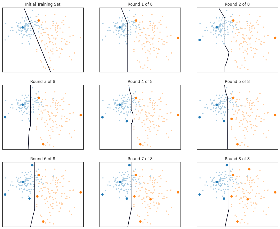
Query the label of the sample that maximizes $u(\mathbf x) = \sum_{h_i \in \mathcal C} D_{\text{KL}}(\hat P_i | \overline P)$. This means the average Kullback-Leibler disagreement between committee members and the consensus is maximized.

def max_disagreement(ensemble: VotingClassifier, X: np.ndarray, train_idx: Sequence[int]) -> int:
  unknown_indices = array([i for i in range(X.shape[0]) if i not in train_idx])

  probas = ensemble._collect_probas(X[unknown_indices])
  consensus = np.mean(probas, axis=0)
  utility = array([
       np.apply_along_axis(entropy, axis=1, arr=probas[:, i], qk=qk).sum()
       for i, qk in enumerate(consensus)
  ])

  return unknown_indices[argmax(utility)]

train_idx = starting_samples[:]
ensemble = VotingClassifier([
  ('logistic regression', LogisticRegression()),
  ('decision tree', DecisionTreeClassifier()),
  ('naive bayes', GaussianNB()),
  ('knn', KNeighborsClassifier(n_neighbors=2))
], voting='soft').fit(X[train_idx], y[train_idx])

figure(figsize=(15, 12))
subplot(3, 3, 1)
title(f'Initial Training Set')
plot_ensemble_voting_decision_boundary(ensemble, X, y, train_idx)
plot_data(X, y, train_idx)

for round in range(8):
  new_sample = max_disagreement(ensemble, X, train_idx)
  train_idx.append(new_sample)

  subplot(3, 3, round+2)
  title(f'Round {round + 1} of 8')
  ensemble = ensemble.fit(X[train_idx], y[train_idx])
  plot_ensemble_voting_decision_boundary(ensemble, X, y, train_idx)
  plot_data(X, y, train_idx)

---

Expected Model Change

• Uncertainty Sampling and Query-by-Committee (QBC) are conceptually similar. You train a model, or an ensemble model, and then use its output on unseen samples to judge the value of each sample. However, this method may select samples close to the decision boundary, and these samples may not always help the model learn the overall structure of the data.

• Expected Model Change (EMC) tries to solve this problem. Its core idea is to look at the future. We no longer ask how uncertain the model is about a sample. Instead, we ask: if we knew the label of this sample, how much would the model change? The samples that can change the model the most are the most valuable samples.

How can we implement Expected Model Change?

The most direct method is to train a model for every possible label, and then compare the difference between the old and new models. However, this method is very expensive and is usually not practical. Fortunately, some methods make this idea more feasible.

For gradient-based optimization methods, such as deep learning, we can use the expected length of the training gradient to approximate the model change. The formula is:

$$
u(x)=\mathbb{E}_y[|\nabla \ell(h ; \ell \cup(x, y))|] \approx \mathbb{E}_y[|\nabla \ell(h ;(x, y))|],
$$

Here, $\ell(h ; \ell)$ is the loss function, and $\ell$ is the training set. This approximation is based on two assumptions:

1. $h$ is an already trained model.

2. The training data are independent and identically distributed.

This means the gradient change only comes from sample $x$ . Therefore, we only need to compute the loss for each $x$, instead of computing it for the whole training set.

In plain language, the core idea of Expected Model Change (EMC) is: select the samples that can change the model the most. Unlike uncertainty sampling and Query-by-Committee, EMC focuses on the future effect of a sample on the model, not the current prediction uncertainty of the model.

import torch
import torch.nn as nn
import torch.optim as optim

# Assume model is an already trained model
# X_unlabeled is the unlabeled dataset

def compute_gradients(model, X_unlabeled):
    gradients = []
    for x in X_unlabeled:
        x = torch.tensor(x, requires_grad=True)
        output = model(x)
        loss = nn.CrossEntropyLoss()(output, model.predict(x))  # Use pseudo-labels
        loss.backward()
        gradients.append(x.grad.norm())  # Compute the gradient norm
    return gradients

def select_samples(model, X_unlabeled, top_k=10):
    gradients = compute_gradients(model, X_unlabeled)
    top_k_indices = torch.topk(torch.tensor(gradients), top_k).indices
    return top_k_indices

---

Expected Error Reduction, EER

Expected Error Reduction aims to select the samples that can reduce the model prediction error on unseen data the most, and then label those samples to improve model performance. The core idea of EER is: select the samples whose labels can significantly reduce the model prediction error on future data.

The core question of EER is: which sample labels can reduce the model prediction error the most?

Idea:

• For each unlabeled sample $x$, assume that we know its true label $y$ as a pseudo-label, and then use this newly labeled sample $(x, y)$ to update the model.
• The updated model will make better predictions on other unlabeled samples $x^{\prime}$, thereby reducing prediction error.
• The goal of EER is to select the samples that can reduce prediction error the most for labeling.

---

Density Weighting

The core idea of density weighting is this: when selecting samples for labeling, we should consider not only model uncertainty, but also how representative each sample is in the data distribution. By combining sample utility with a density estimate, density weighting can avoid selecting samples from sparse regions or outliers.

Density weighting solves the above problem by combining the sample utility $u(x)$ with the density estimate $\hat{p}(x)$ in the feature space. Specifically, the density-weighted utility function is defined as:

$$
u^{\prime}(x)=u(x) \hat{p}(x)^\beta
$$

where:

– $u^{\prime}(x)$ is the adjusted sample utility.

– $\hat{p}(x)$ is the density estimate of sample $x$.

– $\beta$ is a hyperparameter that controls the strength of density weighting.

The main role of density weighting is: to avoid selecting samples from sparse regions of the feature space for labeling. By introducing a density estimate, density weighting ensures that the selected samples are not only highly uncertain, but also representative in the data distribution. This helps avoid outliers and improves the quality of labeled data.

I have a question: is the purpose of active learning not to make training more efficient? But when we search for valuable samples, methods such as EER and EMC seem to require a lot of computation. Is this not against the original goal? Or does active learning have goals beyond computational efficiency, such as making the model more accurate?